Pearls & Plasticine on Plane

Now we will bring a little variance into the shape of our particles. Furthermore, we do not just vary the shape of our one particle kind, but also introduce a second particle type, which distinguishes in shape and color from the first type. The whole scene’s complexity is increased by various feature manipulations.

At a Glance

What We Will Learn

• Inheritance of recipes

• Several particle blueprints with complex geometries

• Assign more realistic materials

• Separately adapt attributes via specified sets

• Add turbidity to the scene

• Learn new render mode categorical

Step 1: Value the Past: Inheritance

As usual, we start by creating a new recipe file – call it plasticine_plane.yaml this time – and add our first block to initialize and seed the recipe. However, instead of starting all over every time when creating a new recipe, this time we’ll make use of another recipe and build upon that. In fact, we take the last one, which we created in the previous tutorial: colPearls_plane.yaml. In order to reference that and build upon it, we easily need to add it to our list of defaults.

plasticine_plane.yaml

# Initializing and seeding
defaults:
  - BaseRecipe
  - colPearls_plane
  - _self_

What we just did, is defining a list of single recipes, where every subsequent recipe builds upon the previous one and adds the content from itself. When specific definitions already existed before, it overwrites that content. In our case, we build upon the BaseRecipe and afterwards add the content of the recipe, which is defined in the file colPearls_plane.yaml (the toolbox synthPIC2 knows that the recipes are located under recipes/.. and we do not need to name the file extension). In the end, we add the content of the current recipe itself by putting the entry _self_ into the list. The current recipe is quite empty at the moment (nothing else than defaults), so actually, we only specified to execute the repice colPearls_plane at the moment. When we currently run our new recipe, we get the same result as if we would run colPearls_plane from the last tutorial.

python run.py --config-dir=recipes --config-name=plasticine_plane

You’re advised to decrease the render samples to a low value like 64 or 128 in this tutorial, if you want to save some time or are bound to hardware limitations. However, we will present those versions of images rendered with 2048 samples throughout the tutorial.

plasticine_plane.yaml

# Physical boundary conditions
process_conditions:
  feature_variabilities:
    CyclesSamples:
      variability:
        value: 64 # small during tutorial, high for final render

As can be seen, we really only needed to add the one value, which we wanted to change, here value: 64 (of course in the namespace tree containing it process_conditions \(\curvearrowright\) feature_variabilities \(\curvearrowright\) CyclesSamples \(\curvearrowright\) variability). That means, this time we didn’t need to specify feature_name: cycles_samples under CyclesSamples: and we didn’t need to specify _target_: $builtins.Constant under variability: again, since those are both already defined in the recipe colPearls_plane from which we inherit and therefore build upon.

One last thing we actually want to change before concluding the first step in this tutorial, is to bring in a new shape: a new geometry prototype for the particles. Therefore, let’s just change this one attribute in its corresponding namespace by adding four lines of code: three for the namespace and one for the attribute geometry_prototype_name, which we want to change.

plasticine_plane.yaml

# Initializing and seeding
defaults:
  - BaseRecipe
  - colPearls_plane
  - _self_
# Defining blueprints
blueprints:
  particles:
    Bead:
      geometry_prototype_name: potato
# Physical boundary conditions
process_conditions:
  feature_variabilities:
    CyclesSamples:
      variability:
        value: 2048 # small during tutorial, high for final render

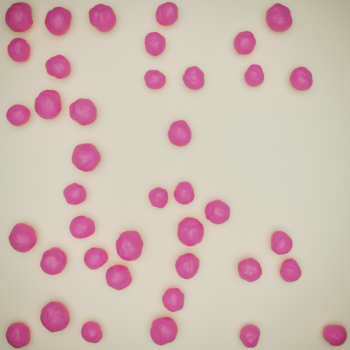
In this first step, we saw how easy it is to create a new recipe based on prior work using the inheritance mechanism of recipes.

Step 2: Playing With Plasticine

Now we introduce a second shape and again want to end up with 40 particles in total.

plasticine_plane.yaml

blueprints:
  particles:
    Bead:
      geometry_prototype_name: potato
      number: 15
    Worm:
      geometry_prototype_name: worm_twisted
      parent: MeasurementVolume
      number: 25

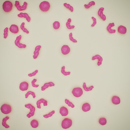
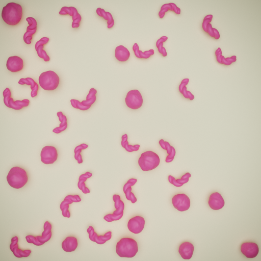
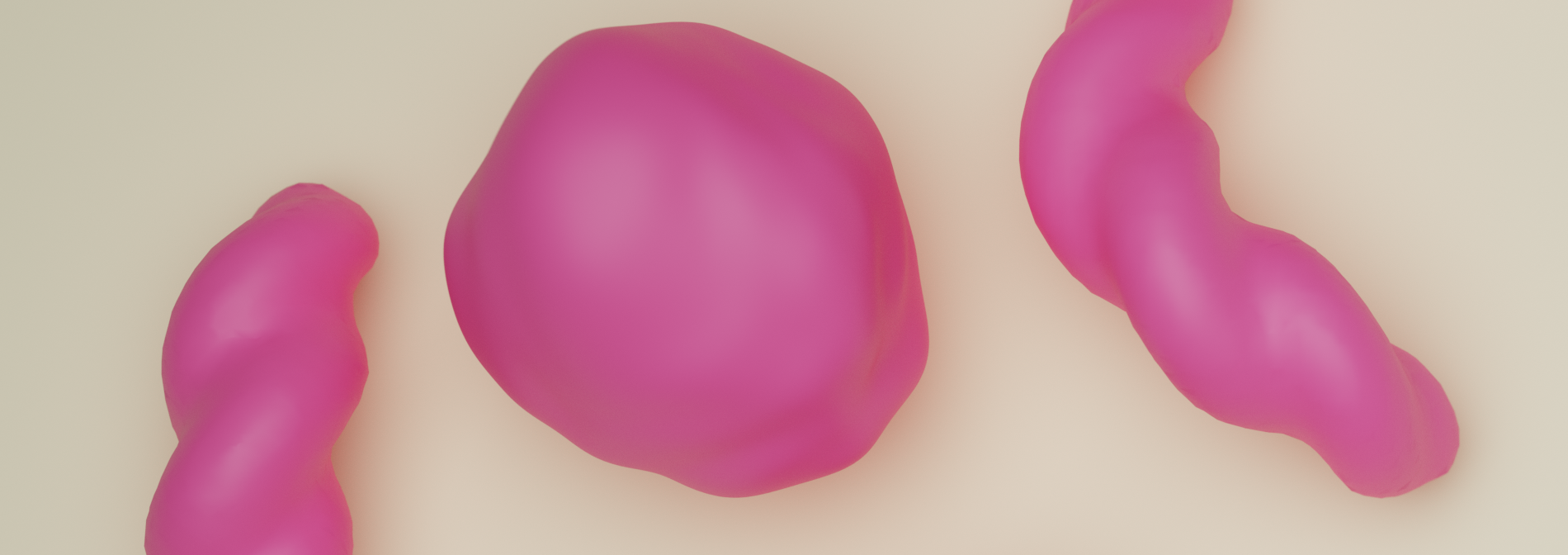
This new shape, which we added, has a worm-like, twisted appearance – something you could achieve by playing with plasticine. We’ll have a look at the possibilities of how to play around with it in a moment. Let’s first visualize our result.

To get an idea what we can do with those plasticine worms, let’s have a look at their geometry prototype: We can find it under prototype_library/geometries/.. in the two files worm_twisted.blend and worm_twisted.yaml. The first describes the geometry in a .blend file, while the second accompanying file specifies the features which are allowed to be changed. Let’s first have a look in the latter.

worm_twisted.yaml

features:
  - name: dimensions …
  - name: location …
  - name: location_z …
  - name: rotations
    blender_link: bpy.data.objects["GeometryPrototype"].modifiers["GeometryNodes"]["Input_2"]
  - name: thickness
    blender_link: bpy.data.objects["GeometryPrototype"].modifiers["GeometryNodes"]["Input_3"]
  - name: resolution
    blender_link: bpy.data.objects['GeometryPrototype'].modifiers["Remesh"].voxel_size

Next to the first three features dimensions, location and location_z (which can also be found, e.g. in the geometry prototype of the sphere), we have three further features for the shape definition of our worms. They are called rotations, thickness and resolution. For the moment, the statements after blender_link: after each feature name can be ignored. For a better – visual – understanding of what we actually change, let’s open the geometry .blend file in Blender.

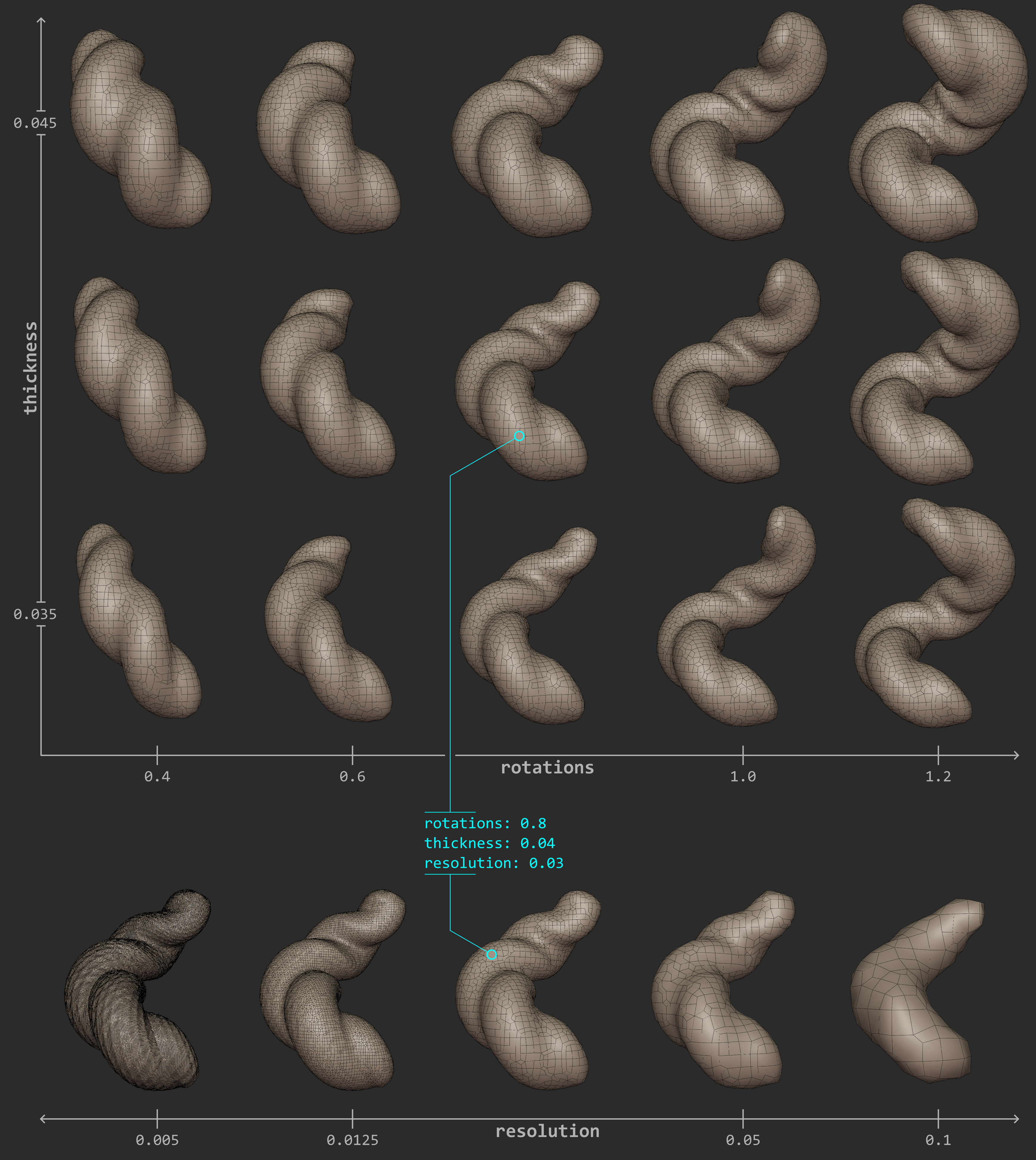
When we now want to adjust those features in our recipe, we define the feature_variabilities and call the TriggerFeatureUpdate as usual. Actually, we do not adjust them directly, but rather define a range, in which those features are allowed to be set during randomization while TriggerFeatureUpdate. So, let’s first define our feature_variabilities under process_conditions. Keep in mind, that we’re still inheriting from the other recipe colPearls_plane and therefore, just need to add/overwrite our desired new elements. However, changing the feature_generation_steps works a little bit different, as we will see soon.

Let’s add the new feature_variabilities, which we call WormRotations, WormThickness and WormResolution, to vary our features (as named in the prototype accompanying file) rotations, thickness and resolution, respectively.

plasticine_plane.yaml

process_conditions:
  feature_variabilities:
    WormRotations:
      feature_name: rotations
      variability:
        _target_: $builtins.UniformDistributionNdHomogeneous
        location: 0.4
        scale: 0.8
    WormThickness:
      feature_name: thickness
      variability:
        _target_: $builtins.UniformDistributionNdHomogeneous
        location: 0.035
        scale: 0.01
    WormResolution:
      feature_name: resolution
      variability:
        _target_: $builtins.Constant
        value: 0.15
    CyclesSamples:
      variability:
        value: 2048 # small during tutorial, high for final render

Via the feature variability named WormResolution, we specified a constant value of 0.15 for the feature resolution of our worms. The other both features were restricted to the allowed intervals as rotations\(\in [0.4,1.2)\) and thickness\(\in [0.035,0.045)\) by their corresponding feature_variabilities named WormRotations and WormThickness, respectively. Now we only need to add the corresponding calls to trigger the update of those features.

However, while we heavily used the concept of inheritance so far, this isn’t quite as easy for the synth_chain, as well. The latter contains only two more attributes which we can add/overwrite, namely the feature_generation_steps and the rendering_steps. When we want to manipulate a specific step below this level, it is not possible to granularly change one element solely by a further recipe in the inheritance chain. The reason for that is that we’re dealing with lists here: A list can only be replaced in its whole. Therefore, in the current version of synthPIC2, when we want to change one or more elements of the feature_generation_steps or the rendering_steps, we need to redefine the whole list. And that is what we do now:

plasticine_plane.yaml

# Procedural steps of synthetization chain
synth_chain:
  feature_generation_steps:
    - _target_: $builtins.InvokeBlueprints
      affected_set_name: AllMeasurementTechniqueBlueprints
    - _target_: $builtins.InvokeBlueprints
      affected_set_name: AllParticleBlueprints
    - _target_: $builtins.TriggerFeatureUpdate
      feature_variability_name: InitialParticleLocation
      affected_set_name: AllParticles
    - _target_: $builtins.TriggerFeatureUpdate
      feature_variability_name: ParticleDimension
      affected_set_name: AllParticles
    - _target_: $builtins.TriggerFeatureUpdate
      feature_variability_name: WormRotations
      affected_set_name: AllParticles
    - _target_: $builtins.TriggerFeatureUpdate
      feature_variability_name: WormThickness
      affected_set_name: AllParticles
    - _target_: $builtins.TriggerFeatureUpdate
      feature_variability_name: WormResolution
      affected_set_name: AllParticles
    - _target_: $builtins.RelaxCollisions
      affected_set_name: AllParticles
      num_frames: 20
      collision_shape: SPHERE
    - _target_: $builtins.RelaxCollisions
      affected_set_name: AllParticles
      use_gravity: True
      damping: 0.07
      friction: 0.4
      restitution: 0.1
      collision_margin: 0.5
      num_frames: 150
      collision_shape: CONVEX_HULL
    - _target_: $builtins.TriggerFeatureUpdate
      feature_variability_name: BackgroundColor
      affected_set_name: AllMeasurementTechniques
    - _target_: $builtins.TriggerFeatureUpdate
      feature_variability_name: PinkColor
      affected_set_name: AllParticles
    - _target_: $builtins.TriggerFeatureUpdate
      feature_variability_name: RenderingResolutionPercentage
      affected_set_name: AllMeasurementTechniques
    - _target_: $builtins.TriggerFeatureUpdate
      feature_variability_name: CyclesSamples
      affected_set_name: AllMeasurementTechniques

Actually, only the highlighted lines differ from those of the last tutorial, i.e. the recipe that we inherit from. However, as described above we need to add the whole list of feature_generation_steps to our new recipe.

As a last detail of shape manipulation, we also want to introduce some variation for our Beads and therefore supply a random value (acting as seed) to the available feature shape of our geometry prototype named potato. Let’s add the new feature variability directly add the top of all feature_variabilities.

plasticine_plane.yaml

process_conditions:
  feature_variabilities:
    BeadShape:
      feature_name: shape
      variability:
        _target_: $plugins.official.UniformDistributionInt
        location: 0
        scale: 10000
    WormRotations: …

We will add the corresponding feature generation step to trigger that feature update right in between our TriggerFeatureUpdate for ParticleDimension and WormRotations.

plasticine_plane.yaml

synth_chain:
  feature_generation_steps:
    - _target_: $builtins.InvokeBlueprints …
    - _target_: $builtins.InvokeBlueprints …
    - _target_: $builtins.TriggerFeatureUpdate …
    - _target_: $builtins.TriggerFeatureUpdate
      feature_variability_name: ParticleDimension
      affected_set_name: AllParticles
    - _target_: $builtins.TriggerFeatureUpdate
      feature_variability_name: BeadShape
      affected_set_name: AllParticles
    - _target_: $builtins.TriggerFeatureUpdate
      feature_variability_name: WormRotations
      affected_set_name: AllParticles

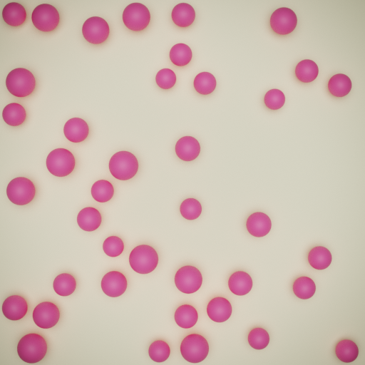
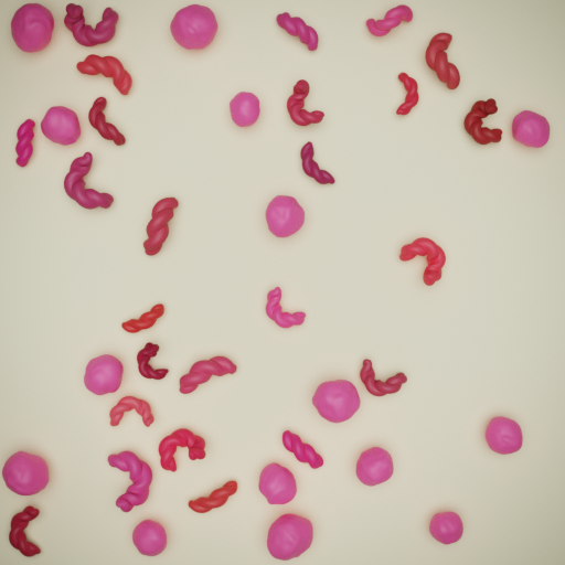
Our rendered image of the scene after adding those variations to shape for our particle types Bead and Worm looks as follows.

Step 3: Richness in Material Details

After we brought in a lot of variation for our particle shapes, i.e. the geometry, we now want to tweak our materials. Two major aspects, which strongly influence the image’s final appearance, are color and texture.

We already have some color in our image, which we inherited from the recipe colPearls_plane. Our particles are pink and the background is beige. Both were defined as a constant, exact color by the HSV color representation. We remember the definitions in our old recipe from the previous tutorial.

colPearls_plane.yaml

process_conditions:
  feature_variabilities:
    InitialParticleLocation: …
    ParticleDimension: …
    RenderingResolutionPercentage: …
    CyclesSamples: …
    BackgroundColor:
      feature_name: color
      variability:
        _target_: $plugins.official.ConstantHsvColorAsRgb
        hue: 0.15
        saturation: 0.35
    PinkColor:
      feature_name: color
      variability:
        _target_: $plugins.official.ConstantHsvColorAsRgb
        hue: 0.95
        saturation: 0.85

We now want to introduce some variation. To be more specific, we want to give the pink color of our particles a little bit more possibilities of appearance – we want to allow the color to spread further into the red area of our color wheel. To better understand what this actually means, expressed in numeric HSV values, let’s bring up the color wheel one more time.

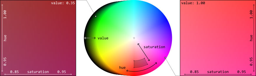
Based on our old pink color with values hue: 0.95, saturation: 0.85 and value: 1.00 (implicitly chosen, since no specification of value defaults to 1.0), we want to extend the range in all these three dimensions. As can be seen in the figure, the two-dimensional range limits of \(0.95\dots 1.00\) for hue and \(0.85\dots 0.95\) for saturation correspond to a segment of an annulus in the color wheel (see dark area). The value, which is plotted in the third dimension, defines the brightness. Note that the little markers in the figure do not indicate the exact color position, but illustrate the value parameter of the HSV representation. To get an idea how strongly we increased the range of possible colors, let’s search for our previous pink color: In the right square – showing the colors for value: 1.00 – our previous pink color sits in the bottom left corner as a fixed color with an exact value. More variation, we didn’t allow by the feature variability named PinkColor from the last tutorial.

Now, we add another feature variability in our new recipe, right below our earlier definitions for the shape features and call it ReddishColor.

plasticine_plane.yaml

feature_variabilities:
  BeadShape: …
  WormRotations: …
  WormThickness: …
  WormResolution: …
  ReddishColor:
    feature_name: color
    variability:
      _target_: $plugins.official.RandomHsvColorAsRgb
      h_min: 0.95
      h_max: 1
      s_min: 0.85
      s_max: 0.95
      v_min: 0.35
      v_max: 1
  CyclesSamples: …

Since we do not want to allow this color variety for all of our particles, but only for our plasticine worms, let’s again control this distinction by sets. This time however, we cannot easily take standard sets (e.g. AllMeasurementTechniques, AllParticles) as we did last time, when we assigned separate background and particle colors. Hence, we need to create two new sets to distinguish our both particle kinds.

The content of sets, i.e. which objects belong to them during runtime, is defined by logical combination of criteria. Let’s think about it: What is our criterion for distinction? The difference between a Bead and a Worm… They are different particle types, defined by different blueprints! So let’s take this criterion: The distinction by their origin and filter for their blueprints’ name. We create two new feature_criteria and two corresponding sets under our process_conditions. Let’s add them before our feature_variabilities.

plasticine_plane.yaml

process_conditions:
  feature_criteria:
    IsBead:
      _target_: $builtins.ContainsString
      feature_name: blueprint_name
      search_string: Bead
      default_return_value: False
    IsWorm:
      _target_: $builtins.ContainsString
      feature_name: blueprint_name
      search_string: Worm
      default_return_value: False
  sets:
    BeadsInView:
      criterion: $IsParticle and $IsBead
    WormsInView:
      criterion: $IsParticle and $IsWorm
  feature_variabilities:
    BeadShape: …
    WormRotations: …
    WormThickness: …
    WormResolution: …
    ReddishColor: …
    CyclesSamples: …

Everything is prepared now to assign the colors (more exactly: the allowed color variabilities) to our desired particles, based on their affiliation to a certain set. This assignment will be evaluated during runtime, i.e. the evaluation which particle belongs to which set happens when the concrete feature_generation_step is executed. We add the new TriggerFeatureUpdate for our feature_variability with name ReddishColor right below our other both feature_generation_steps, which trigger the update of the feature color according to the feature_variabilities named BackgroundColor and PinkColor.

plasticine_plane.yaml

    - _target_: $builtins.TriggerFeatureUpdate
      feature_variability_name: BackgroundColor
      affected_set_name: AllMeasurementTechniques
    - _target_: $builtins.TriggerFeatureUpdate
      feature_variability_name: PinkColor
      affected_set_name: BeadsInView
    - _target_: $builtins.TriggerFeatureUpdate
      feature_variability_name: ReddishColor
      affected_set_name: WormsInView

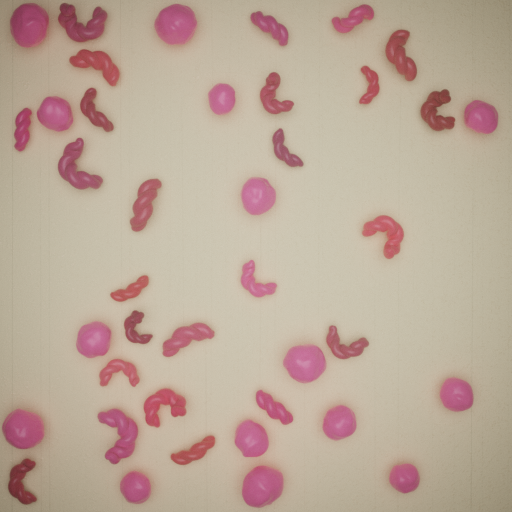
Note that we also adjusted our already existing TriggerFeatureUpdate for PinkColor by changing the affected_set_name to our newly created set BeadsInView. Executing the recipe at the current state outputs a rendered image with all Beads still having their fixed pink color, while our plasticine Worms show a reddish tint. Most importantly, all Worms have a different, unique (randomized) color, which was defined/restricted by the feature_variability named ReddishColor.

As a last measure to conclude the current step of this tutorial: We’ll tune the materials! This can easily be done by adding the following five lines to our blueprints section.

plasticine_plane.yaml

blueprints:
  measurement_techniques:
    TopCamInAir:
      background_material_prototype_name: cracks_subtle
  particles:
    Bead:
      geometry_prototype_name: potato
      material_prototype_name: colored_subtle
      number: 15
    Worm:
      geometry_prototype_name: worm_twisted
      material_prototype_name: colored_subtle
      parent: MeasurementVolume
      number: 25

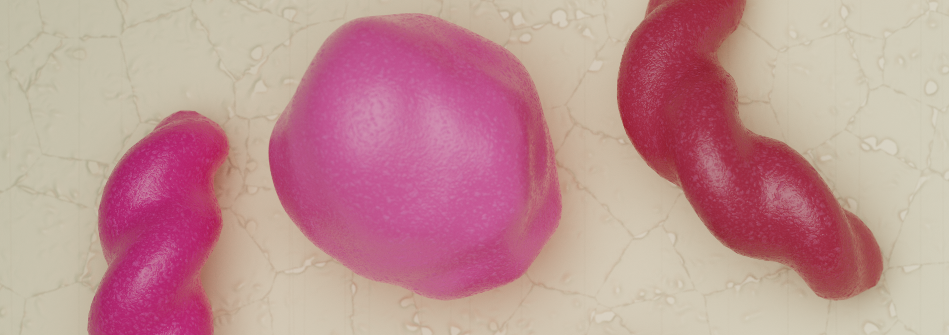
We defined the both materials cracks_subtle and colored_subtle for our background and for our particles, respectively. As the names suggest, those materials show only a subtle nuance of structure, but add more realism to the scene than the previous plain materials could do. Those more complex materials make use of procedurally generated textures and show little, but clear difference especially in the specular highlights, see rendered image.

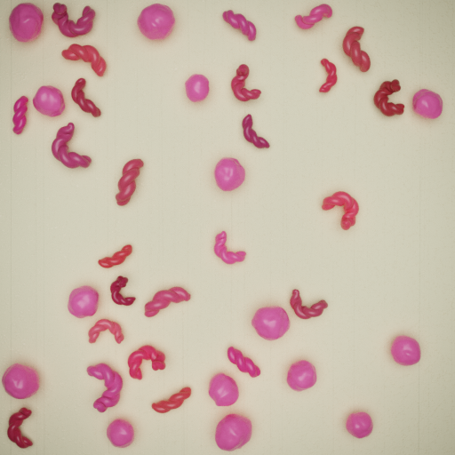
Step 4: Clear Vision in Fog

In this last step of our tutorial, we add that little salt and pepper to our scene. Namely, we want to add some turbidity to our vision: a homogeneous fog. When looking at our last rendered images: They all look sharp… very crisp. Nice, but not very realistic. In practice, there’s often at least some extent of blur in recorded images of particles by dust or the like (participating media) in the measurement volume. Our measurement_technique named TopCamInAir with its geometry prototype (defined in measurement_technique_prototype_name) named plane_topCam_fog already contains that property. We just have to turn it on! Let’s add another feature variability, which defines the feature fog. We’ll name it MeasurementVolumeFog.

plasticine_plane.yaml

  feature_variabilities:
    BeadShape: …
    WormRotations: …
    WormThickness: …
    WormResolution: …
    ReddishColor: …
    MeasurementVolumeFog:
      feature_name: fog
      variability:
        _target_: $builtins.Constant
        value: 0.025
    CyclesSamples: …

Again, we also need to add the corresponding TriggerFeatureUpdate as a new feature_generation_step. We add it right in between the TriggerFeatureUpdates for ReddishColor and RenderingResolutionPercentage.

plasticine_plane.yaml

    - _target_: $builtins.TriggerFeatureUpdate
      feature_variability_name: ReddishColor
      affected_set_name: WormsInView
    - _target_: $builtins.TriggerFeatureUpdate
      feature_variability_name: MeasurementVolumeFog
      affected_set_name: AllMeasurementTechniques
    - _target_: $builtins.TriggerFeatureUpdate
      feature_variability_name: RenderingResolutionPercentage
      affected_set_name: AllMeasurementTechniques

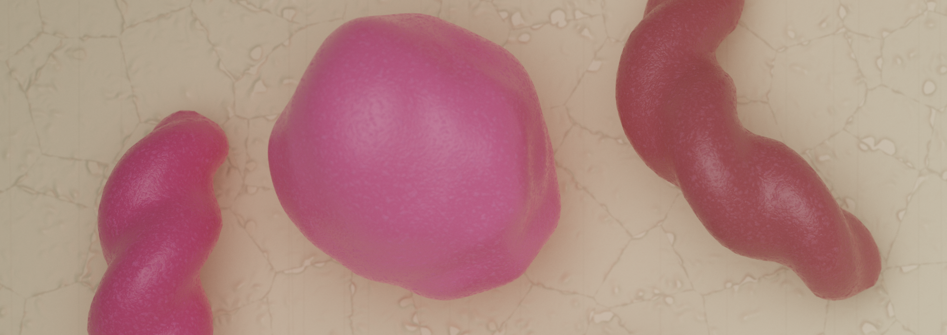
The addition of this fog (technically: volume scatter) to our scene will result in a higher render time / higher number of needed samples for an output image with a satisfyingly low amount of noise. Therefore, you should always carefully consider if volume scattering is really needed for the concrete use case.

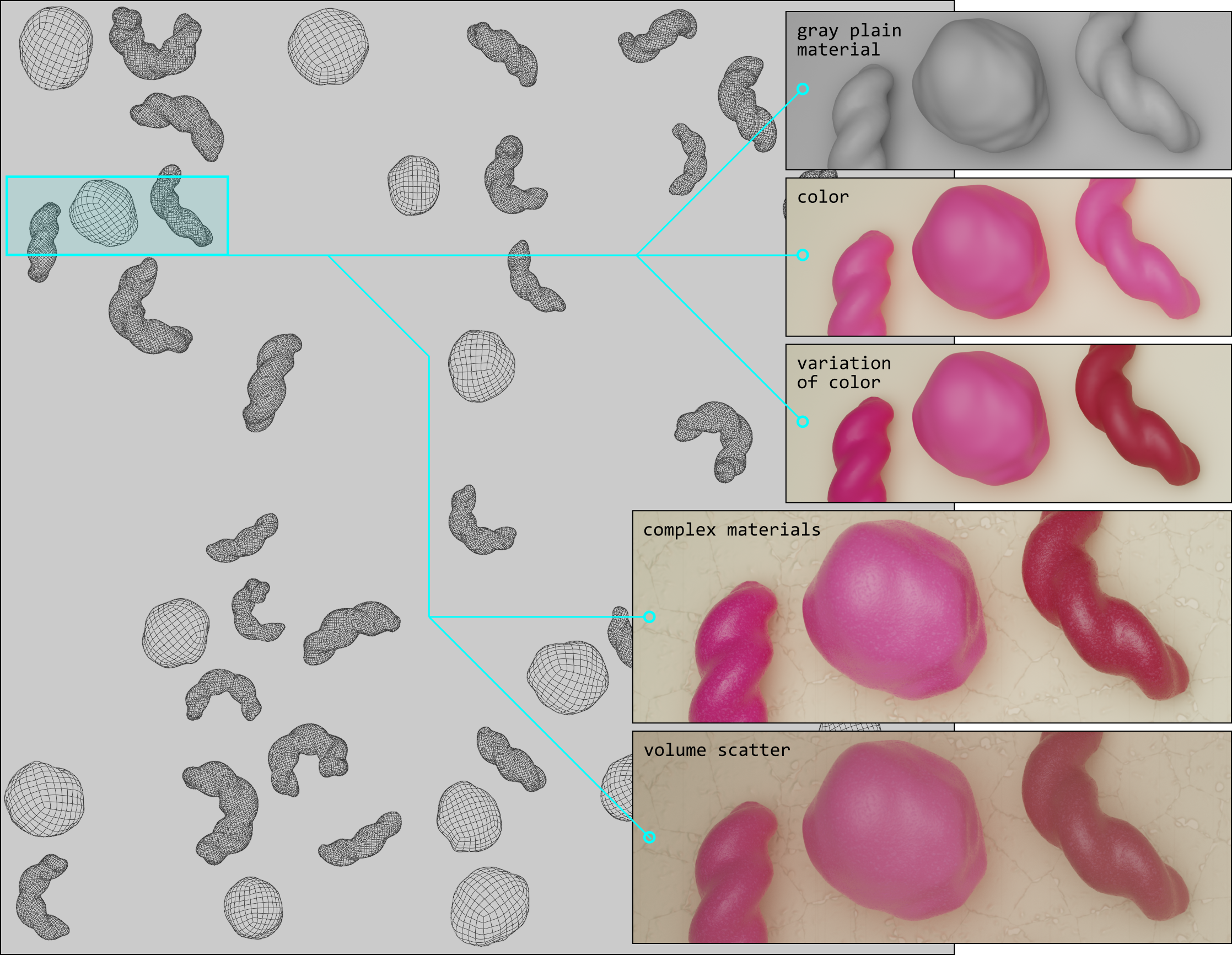
Up to this point, we put quite a lot of effort into rendering an image that represents the synthesized image in an appearance similar to that taken by a real photo camera. Let’s recap our steps to increase the complexity of the scene, for a moment.

First, we added color to the simple material plain and then introduced color variation in a specific range for one type of our particles. Afterwards, we increased the complexity by choosing new materials, which also contain a feature named color. Therefore we kept our currently chosen color for the particles, but just added a subtle texture with the new material. As a last step, we added a very low amount of volume scatter to simulate a fine fog.

High resolution images (click to enlarge):

To conclude this tutorial, we want to have a look at another rendering_mode called categorical. Let’s first start by actually creating a rendering_steps list and adding our “normal” rendering_step to output the real image. Afterwards, we add two new rendering_steps with rendering_mode: categorical.

plasticine_plane.yaml

  rendering_steps:
    - _target_: $builtins.RenderParticlesTogether
      rendering_mode: real
      do_save_features: True
    - _target_: $builtins.RenderParticlesTogether
      rendering_mode: categorical
    - _target_: $builtins.RenderParticlesIndividually
      rendering_mode: categorical
      subfolder: individual

The first categorical step targets the function RenderParticlesTogether to render all particles on one image. So far, for our recently created images with rendering_mode: real, we used this function all the time. This function causes that areas of rear particles, where front particles overlap those, are occluded. In the second categorical step, we want to render each particle on one separate image while neglecting the existence of other particles. This will output all pixels of each specific particle, regardless of the existence of other particles, which would actually overlap those areas. However, in our example here, we do not have overlapping particles anyways, so the RenderParticlesTogether step is the most senseful here.

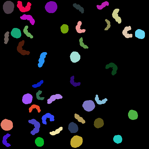
Particles, which are each individually rendered on one image, are placed in the subfolder whose name we specified as individual. Six example images are shown here.

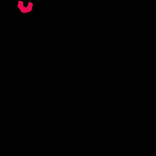
For this mode categorical, the earlier defined CyclesSamples are of no importance. We see no details of the photo-realistic appearance, for which we put quite a lot of effort into the creation of our recipe. However, this mode brings something very valuable: We exclusively see the plain and simple exact pixel coordinates, color-coded with their belonging to each particle. The location with exact boundary (i.e. shape) and therefore the two-dimensional size are unambiguously described for each single particle. A very valuable knowledge of the ground truth in our images, e.g. for generation of training data for neural networks.

In the fourth line of the last code snipped we stated do_save_features: True. By this, the additional files measurement_technique_features.csv and particle_features.csv are output in the corresponding subfolder of the rendering_step. The latter of the two files contains all features for all particles, including the category_color of each particle. Therefore, especially when using the categorical render mode, at least one of the rendering_steps should also output these files by setting do_save_features: True. So, further data sorting and assignability of each particle with its features to the color-coded location on the categorical image is made possible.

As you can see, the term “rendering” is used in synthPIC2 in a more general context. While in the context of computer graphics, it often directly means the generation of an image. We rather define it in the context of translating features from our virtual reality (3D measurement volume) domain into an explicit format. This can be a numeric table, a photo-realistically rendered image, categorical images or also the full geometrical data of each particle, i.e. the mesh data.