Chocolate Beans on Table
In this tutorial, we’ll extend our workflow by including the generation of a prototype. Based on the previous basic tutorials, our starting scene will be similar: We generate pink pearls on a plane and step-by-step increase the complexity of the scene. A more in-depth use of our beloved RelaxCollisions function will introduce the dry_run mode.
At a Glance
What We Will Learn
Create a new, own prototype
Illuminate the scene by HDRI light
Create different particle classes
Color definition in HSV representation
Specify particles based on dynamic sets
Step 1: Prepare a Clean Start
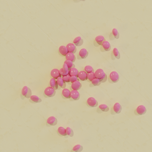
Let’s put aside those plasticines and deformed particles. We want to start this time, by a clean and simple scene with pink pearls: Create a new recipe and call it chocBeans_table.yaml. Our first code snippet, as usual, will initialize and seed the recipe.
# Initializing and seeding
defaults:
  - BaseRecipe
  - _self_
initial_runtime_state:
  seed: 42
We want to start with a similar scene like last time, choosing the cracks_subtle material for our background and the colored_subtle material for our particles. However, the measurement technique used in this tutorial will be another one, called woodTable_sideCam.
# Defining blueprints
blueprints:
  measurement_techniques:
    TopCamInAir:
      measurement_technique_prototype_name: woodTable_sideCam
      background_material_prototype_name: cracks_subtle
  particles:
    Bead:
      geometry_prototype_name: sphere
      material_prototype_name: colored_subtle
      number: 40
As the name of the measurement technique suggests, we need to slightly adjust the camera angle. Doing so, let’s directly add our other process_conditions, as well.
# Physical boundary conditions
process_conditions:
  feature_variabilities:
    CameraAltitude:
      feature_name: cam_altitude
      variability:
        _target_: $builtins.Constant
        value: 0.96
    InitialParticleLocation:
      feature_name: location
      variability:
        _target_: $builtins.UniformlyRandomLocationInMeasurementVolume
    ParticleDimension:
      feature_name: dimensions
      variability:
        _target_: $builtins.UniformDistribution3dHomogeneous
        location: 3.58
        scale: 0.6
    RenderingResolutionPercentage:
      feature_name: resolution_percentage
      variability:
        _target_: $builtins.Constant
        value: 25
    CyclesSamples:
      feature_name: cycles_samples
      variability:
        _target_: $builtins.Constant
        value: 64
Now we can build our synth chain by starting with the invocation of our blueprints. Afterwards, we trigger of the updates for our features cam_altitude, location and dimensions, which are allowed in the ranges CameraAltitude, InitialParticleLocation and ParticleDimension, respectively.
# Procedural steps of synthetization chain
synth_chain:
  feature_generation_steps:
    - _target_: $builtins.InvokeBlueprints
      affected_set_name: AllMeasurementTechniqueBlueprints
    - _target_: $builtins.InvokeBlueprints
      affected_set_name: AllParticleBlueprints
    - _target_: $builtins.TriggerFeatureUpdate
      feature_variability_name: CameraAltitude
      affected_set_name: AllMeasurementTechniques
    - _target_: $builtins.TriggerFeatureUpdate
      feature_variability_name: InitialParticleLocation
      affected_set_name: AllParticles
    - _target_: $builtins.TriggerFeatureUpdate
      feature_variability_name: ParticleDimension
      affected_set_name: AllParticles
Since again, we want to distribute particles laying flat on a plane, we use the RelaxCollisions function two times, as we did in our previous tutorials. First, to get rid of intersections. A second call – with gravity enabled – to bring all particles onto the ground level.
synth_chain:
  feature_generation_steps:
    - _target_: $builtins.InvokeBlueprints …
    - _target_: $builtins.InvokeBlueprints …
    - _target_: $builtins.TriggerFeatureUpdate …
    - _target_: $builtins.TriggerFeatureUpdate …
    - _target_: $builtins.TriggerFeatureUpdate …
    - _target_: $builtins.RelaxCollisions
      affected_set_name: AllParticles
      num_frames: 5
      time_scale: 10
      collision_shape: CONVEX_HULL
    - _target_: $builtins.RelaxCollisions
      affected_set_name: AllParticles
      use_gravity: True
      damping: 0.1
      friction: 0.999
      restitution: 0.001
      collision_margin: 0.001
      num_frames: 200
      collision_shape: CONVEX_HULL
The last ingredients, we add to our recipe are two more elements in the list of feature_generation_steps and one step for the list of rendering_steps.
synth_chain:
  feature_generation_steps:
    - _target_: $builtins.InvokeBlueprints …
    - _target_: $builtins.InvokeBlueprints …
    - _target_: $builtins.TriggerFeatureUpdate …
    - _target_: $builtins.TriggerFeatureUpdate …
    - _target_: $builtins.TriggerFeatureUpdate …
    - _target_: $builtins.RelaxCollisions …
    - _target_: $builtins.RelaxCollisions …
    - _target_: $builtins.TriggerFeatureUpdate
      feature_variability_name: RenderingResolutionPercentage
      affected_set_name: AllMeasurementTechniques
    - _target_: $builtins.TriggerFeatureUpdate
      feature_variability_name: CyclesSamples
      affected_set_name: AllMeasurementTechniques
  rendering_steps:
    - _target_: $builtins.RenderParticlesTogether
      rendering_mode: real
      do_save_features: True
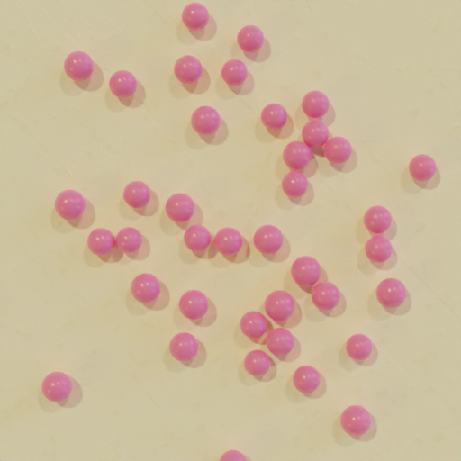
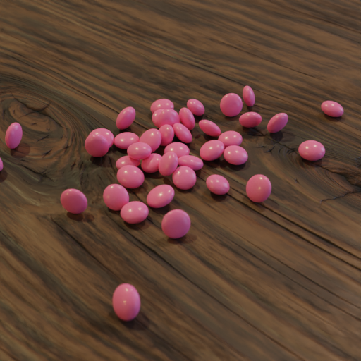
Now we have our whole recipe together for a clean, basic start. Let’s execute it!
python run.py --config-dir=recipes --config-name=chocBeans_table
Since, you very attentively followed the tutorial, instead of just copy-pasting the code snippets, you rightly ask yourself: “Why is there color?” The answer is: It sits in the both material prototypes and we’re looking at their default colors. It just coincidentally happens to be the color of our previous tutorials: pink for the particles, beige for the background. Pretty!
Some more little changes we notice. There is no gap between the particles – see parameter collision_margin: 0.001 of our second RelaxCollisions function – and one particle at the bottom is almost out of our field of view. The latter is caused by another bounding box than that used in earlier tutorials, i.e. the MeasurementVolume, which limits our particles’ spatial distribution for this loaded measurement technique prototype. Furthermore, we notice the two shadows of each particle and will come to the explanation later.
As a last measure, let’s add the material prototype for our measurement volume and the parent of our particle blueprint Bead. This doesn’t change the appearance of the scene, but is just good practice for completion of our recipe at this stage.
blueprints:
  measurement_techniques:
    TopCamInAir:
      measurement_technique_prototype_name: woodTable_sideCam
      measurement_volume_material_prototype_name: vacuum
      background_material_prototype_name: cracks_subtle
  particles:
    Bead:
      geometry_prototype_name: sphere
      material_prototype_name: colored_subtle
      parent: MeasurementVolume
      number: 40
Step 2: Our Own Offspring
In this step, we will actually create a new geometry prototype for our particle blueprint Bead, integrate it in our recipe and manipulate some features of it. Keep in mind that this is not a Blender tutorial, so we’ll barely scratch the surface of that wonderful tool. Rather, we introduce the general idea of integrating a new geometry prototype to our toolbox synthPIC2.
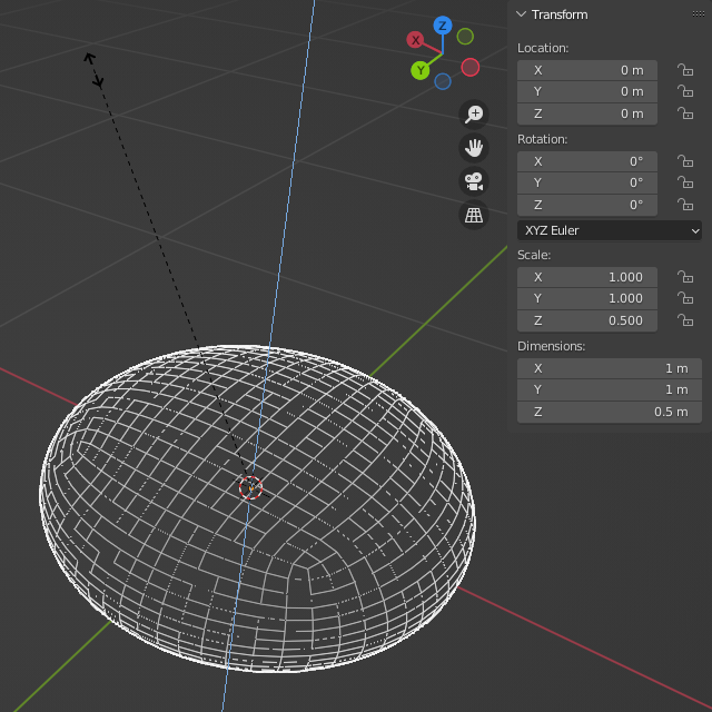
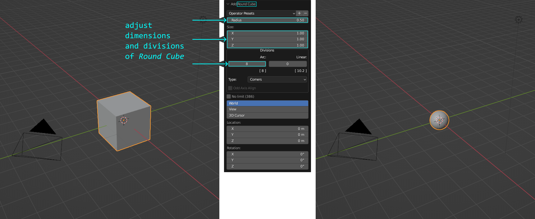
Let’s first start by opening Blender with a new default General scene. We delete the default cube and add a Mesh > Round Cube. As Radius we specify 0.5 and a Size of 1.0 in all three spatial dimensions X, Y and Z. In general, we want our prototypes to have a basic spatial extent of 1.0 in all directions to achieve size consistency across multiple geometry prototypes. For Divisions, we define a number of 8 for Arc as sufficient.
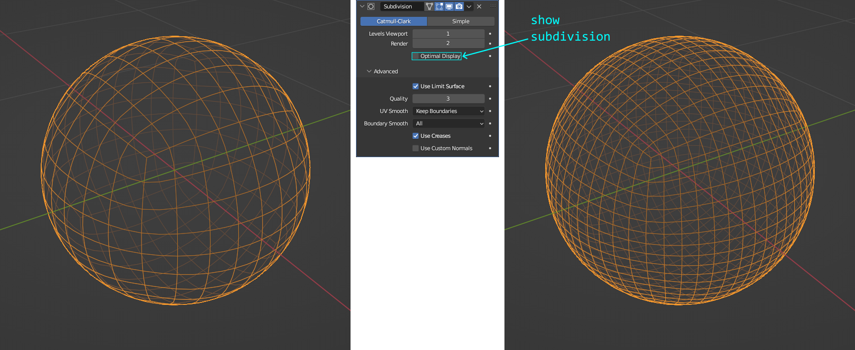
Next, we want to change the faces’ appearance of our geometry. Therefore, we set Shade Smooth (right click on object), which renders and displays faces smooth, using interpolated vertex normals. Furthermore, let’s add a Subdivision Surface modifier and keep all the settings as their default values. This will set the Catmull-Clark algorithm with 1 subdivision level for the viewport and a level of 2 for the final render. The Subdivision Surface modifier gives us a great opportunity to later on – during the execution of our SynthRecipe in synthPIC2 – change the resolution of our particle geometry.
We want to create a prototype that represents an ellipsoid. So, let’s scale it along the Z axis by a factor of 0.5. Basically, this should just obviously show that this prototype represents an ellipsoid – we’ll anyways make this parameter available as a feature to enable a manipulation directly in synthPIC2. As per definition for a geometry prototype, we also need to rename the object of interest in our scene, which is still called Roundcube. The concrete name must be GeometryPrototype for synthPIC2 to identify it.
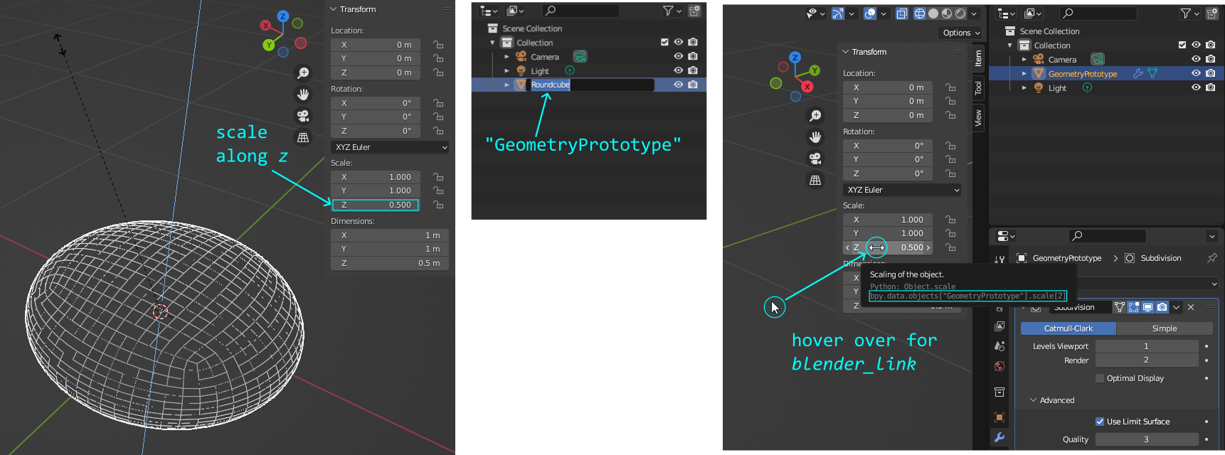
Now let’s introduce the flexibility: We will give synthPIC2 access to change any feature, for which we want to allow a manipulation. To do so, you must first setup Blender to display the blender_link, which we need in synthPIC2. Therefore, in Blender go to Edit > Preferences... > Interface > Tooltips and enable the option Python Tooltips. Now, when you hover over (almost) any menu entry in the GUI of Blender, you will see the address of that concrete parameter in Python with its namespace. It reads something like, e.g. bpy.data.objects… and equals the entry, which we need for our accompanying yaml file of each prototype. You can easily copy this concrete link of a specific feature within Blender by right-clicking on it and then select Copy Full Data Path.
The name of a feature for synthPIC2, which represents the blender_link, can be freely chosen. But keep in mind! Features can be manipulated completely flexible across all invoked blueprints, independent if the feature, e.g. color origins from the material prototype of a particle or the measurement volume material or the background material of the measurement technique or if it origins from any geometry prototype. Once invoked, every object of the scene possesses those features with the names defined in their corresponding prototypes. Therefore, you should establish some rules for generic feature names and exclusive feature names to make use of this powerful capability of synthPIC2 to change all kinds of features across all objects in the scene at once – if wanted and constrainable to specific groups of objects by sets.
Now that we know how to do it: Let’s actually take some parameters in Blender and define those to become our manipulable features in synthPIC2!
First, we save the modeled geometry prototype for our ellipsoid. We need to place it in the location prototype_library/geometries/ and give the name ellipsoid.blend. For the accompanying file, we create a new file with name ellipsoid.yaml and place it in the same directory. Let’s add the following lines to that accompanying file to make manipulation of these features available in synthPIC2.
features:
  - name: dimensions
    blender_link: bpy.data.objects["GeometryPrototype"].dimensions
  - name: width
    blender_link: bpy.data.objects["GeometryPrototype"].scale[1]
  - name: height
    blender_link: bpy.data.objects["GeometryPrototype"].scale[2]
  - name: location
    blender_link: bpy.data.objects["GeometryPrototype"].location
  - name: location_z
    blender_link: bpy.data.objects["GeometryPrototype"].location.z
  - name: subdivisions
    blender_link: bpy.data.objects["GeometryPrototype"].modifiers["Subdivision"].render_levels
Finally, let’s bring it into our scene, that new prototype! To do so, within our SynthRecipe, we need to change the geometry_prototype_name of our Bead.
blueprints:
  measurement_techniques: …
  particles:
    Bead:
      geometry_prototype_name: ellipsoid
      material_prototype_name: colored_subtle
      parent: MeasurementVolume
      number: 40
We also want to see the change of some parameters! So let’s play with the height. To see an obvious effect, we try a weird shape with a height that is three times the width of the ellipsoid by adding a new feature variability called ParticleHeight.
process_conditions:
  feature_variabilities:
    CameraAltitude: …
    InitialParticleLocation: …
    ParticleDimension: …
    ParticleHeight:
      feature_name: height
      variability:
        _target_: $builtins.Constant
        value: 3
Furthermore, we add the corresponding feature_generation_step to trigger the feature update.
synth_chain:
  feature_generation_steps:
    - _target_: $builtins.InvokeBlueprints …
    - _target_: $builtins.InvokeBlueprints …
    - _target_: $builtins.TriggerFeatureUpdate …
    - _target_: $builtins.TriggerFeatureUpdate
      feature_variability_name: InitialParticleLocation
      affected_set_name: AllParticles
    - _target_: $builtins.TriggerFeatureUpdate
      feature_variability_name: ParticleDimension
      affected_set_name: AllParticles
    - _target_: $builtins.TriggerFeatureUpdate
      feature_variability_name: ParticleHeight
      affected_set_name: AllParticles
An execution of the recipe will give us a – yes, let’s call it a weird – shape of our ellipsoidal particles, which obviously differs from the sphere.
Keep in mind that we already triggered the updates of our features location and dimensions within their allowed ranges InitialParticleLocation and ParticleDimension, respectively for these ellipsoids. We did so by choosing the appropriate feature names, when we defined the features in the accompanying file ellipsoid.yaml. So, since we kept to those naming conventions, we didn’t need to adjust anything else in the recipe.
Okay, that works. Now let’s go more in the direction of a usual shape for a chocolate bean. We create a further feature variability for the feature width and also adapt the recent one for the feature height. Both shall be allowed within a certain range instead of only defining a specific constant.
process_conditions:
  feature_variabilities:
    CameraAltitude: …
    InitialParticleLocation: …
    ParticleDimension: …
    ParticleWidth:
      feature_name: width
      variability:
        _target_: $builtins.UniformDistributionNdHomogeneous
        location: 0.85
        scale: 0.15
        num_dimensions: 1
    ParticleHeight:
      feature_name: height
      variability:
        _target_: $builtins.UniformDistributionNdHomogeneous
        location: 0.475
        scale: 0.15
        num_dimensions: 1
We only need to add the TriggerFeatureUpdate for ParticleWidth now.
synth_chain:
  feature_generation_steps:
    - _target_: $builtins.InvokeBlueprints …
    - _target_: $builtins.InvokeBlueprints …
    - _target_: $builtins.TriggerFeatureUpdate …
    - _target_: $builtins.TriggerFeatureUpdate …
    - _target_: $builtins.TriggerFeatureUpdate
      feature_variability_name: ParticleDimension
      affected_set_name: AllParticles
    - _target_: $builtins.TriggerFeatureUpdate
      feature_variability_name: ParticleWidth
      affected_set_name: AllParticles
    - _target_: $builtins.TriggerFeatureUpdate
      feature_variability_name: ParticleHeight
      affected_set_name: AllParticles
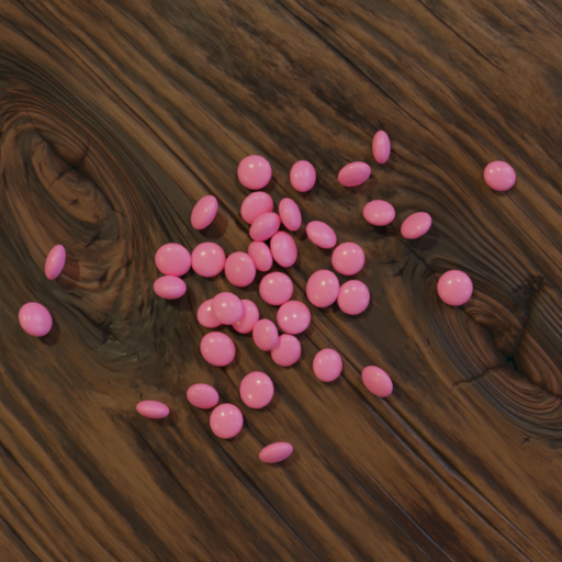
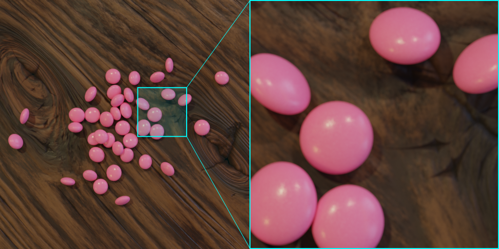
The currently rendered image looks more like ellipsoids in the shape of chocolate beans.
Step 3: Material, Light and Perspective
We’re getting closer! Now, let’s tune it a little bit and slightly change the behavior of how the particles fall: We’ll only turn down the damping of the second RelaxCollisions function just a little bit.
    - _target_: $builtins.RelaxCollisions
      affected_set_name: AllParticles
      num_frames: 5
      time_scale: 10
      collision_shape: CONVEX_HULL
    - _target_: $builtins.RelaxCollisions
      affected_set_name: AllParticles
      use_gravity: True
      damping: 0.07
      friction: 0.999
      restitution: 0.001
      collision_margin: 0.001
      num_frames: 200
      collision_shape: CONVEX_HULL
Furthermore, we change the material of our background to a material named wood.
blueprints:
  measurement_techniques:
    TopCamInAir:
      measurement_technique_prototype_name: woodTable_sideCam
      measurement_volume_material_prototype_name: vacuum
      background_material_prototype_name: wood
The currently rendered image placed our particles more in the right light. Speaking of light, we wanted to have a closer look on how our scene is actually illuminated. Why is there more than one shadow? Why do we see several specular reflections in the particles?
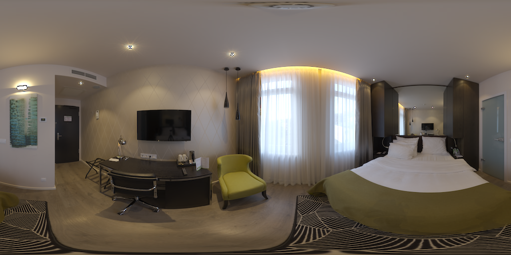
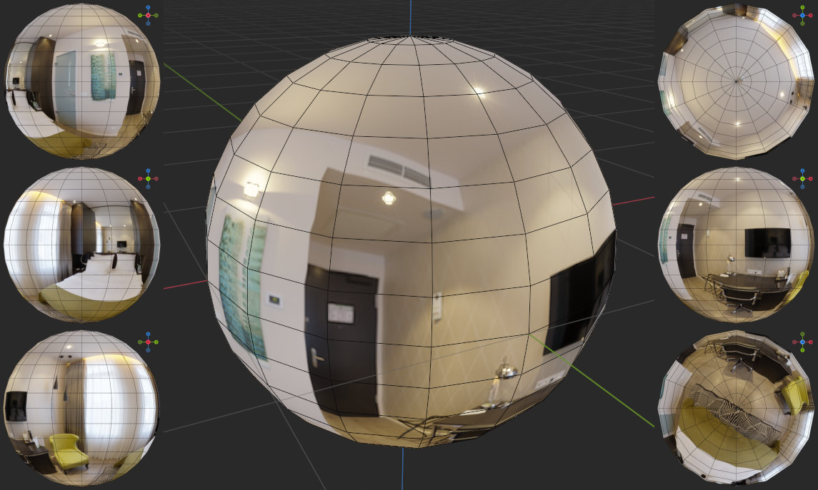
The answer lies in the way of how the scene is illuminated. In the chosen measurement technique prototype named woodTable_sideCam, the scene is illuminated by an HDRI. You can have a look at this by opening the file woodTable_sideCam.blend in Blender and check World Properties > Surface > Background > Color > Color > Image > interior.exr. The last filename is actually the name of the HDRI file, which is shown in the following image.
We’re looking at an HDRI spherical panorama image. HDRI (High Dynamic Range Imaging) stands for a technique that combines images – usually multiple shots at various exposure times – to output a file with increased pixel depth / dynamic range. EXR and HDR are the industry standard file formats to store the data.
In the following figure, this image is plotted onto a UV sphere. You can imagine that the same happens to our scene: We’re sitting just right in the middle of such a big ball and looking at the outside with that big image projected everywhere around us. The light, which illuminates every detail in our scene comes from the surrounding sphere and is represented in location, brightness and color by the corresponding pixels of the HDRI. The HDRI used here is part of the standard HDRIs, which are deployed with Blender.
The next thing we do, is changing the perspective. Instead of looking from the top onto our wooden table with chocolate beans, this time, we want to watch the scene from the side. To achieve this, we will change some features of our measurement technique. We will not need the feature variability for our feature cam_altitude any longer, since the default value of the measurement technique prototype already fits our wanted perspective well. Let’s therefore completely replace the code block for CameraAltitude with a new one called CameraNearTable.
process_conditions:
  feature_variabilities:
    CameraNearTable:
      feature_name: cam_location_z
      variability:
        _target_: $builtins.Constant
        value: -35.0
    InitialParticleLocation:
      feature_name: location
      variability:
        _target_: $builtins.UniformlyRandomLocationInMeasurementVolume
We also need to change the feature_variability_name of the corresponding TriggerFeatureUpdate. Afterwards, we can execute the recipe and admire our rendered image with a view at the scene from this new perspective.
synth_chain:
  feature_generation_steps:
    - _target_: $builtins.InvokeBlueprints …
    - _target_: $builtins.InvokeBlueprints
      affected_set_name: AllParticleBlueprints
    - _target_: $builtins.TriggerFeatureUpdate
      feature_variability_name: CameraNearTable
      affected_set_name: AllMeasurementTechniques
    - _target_: $builtins.TriggerFeatureUpdate
      feature_variability_name: InitialParticleLocation
      affected_set_name: AllParticles
Step 4: Categories and Color
Okay, pink. Pink is nice. But looking at our title: Chocolate beans was the idea… Those usually come in different colors.
In order to assign different colors to different particles, we will use – I think you already guessed – features. We will use the feature color and assign an HSV value, the same way as we did in the previous tutorials. This time however, we want to differentiate between particles, which were invoked from the same blueprint. Therefore, in order to purposefully distinguish between the individual particles with the help of sets, we need to find another criterion for our current case. Doing so, we will discover the dynamic character of sets…
We want to distinguish between single particles by their feature location_z. To better understand why we choose this feature, we could open the measurement technique prototype in Blender and observe how the MeasurementVolume is setup to bound the distribution of the particles in the volume of the 3D virtual scene. However, rather than opening the measurement technique prototype, let’s open the result of our current recipe execution to actually see the particles distributed in the volume!
To do so, we need to add two more elements to our synth_chain. First, we add the parameter dry_run to our second RelaxCollisions function step of the feature_generation_steps and set it to True.
    - _target_: $builtins.RelaxCollisions
      affected_set_name: AllParticles
      num_frames: 5
      time_scale: 10
      collision_shape: CONVEX_HULL
    - _target_: $builtins.RelaxCollisions
      affected_set_name: AllParticles
      use_gravity: True
      damping: 0.07
      friction: 0.999
      restitution: 0.001
      collision_margin: 0.001
      num_frames: 200
      collision_shape: CONVEX_HULL
      dry_run: True
Second, we add a new element to our list of rendering_steps to output a blend file of the scene, after the recipe ran through all feature_generation_steps – another type of rendering, i.e. translating features from our virtual scene into an explicit format.
  rendering_steps:
    - _target_: $builtins.SaveState
      name: state
    - _target_: $builtins.RenderParticlesTogether
      rendering_mode: real
      do_save_features: True
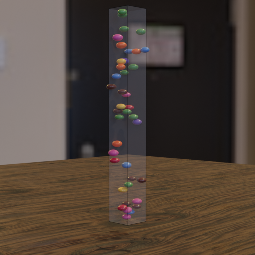
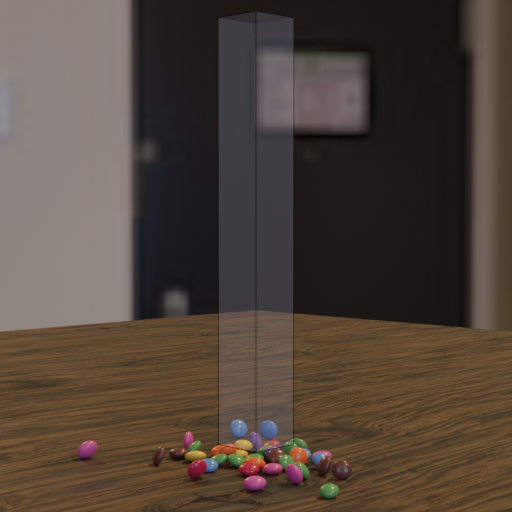
Now, we open that file in Blender, which can be found under output/chocBeans_table/<YYYY-MM-DD_hh-mm-ss>/run0/state.blend – ignore the Glass for a moment in joyful anticipation for the next tutorial – and have a look at the particles being distributed in the virtual scene. The advantage of using the parameter dry_run is that we can visualize every frame of the RelaxCollisions simulation, meaning: our falling particles. The images below show the first frame and the last frame of this simulation.
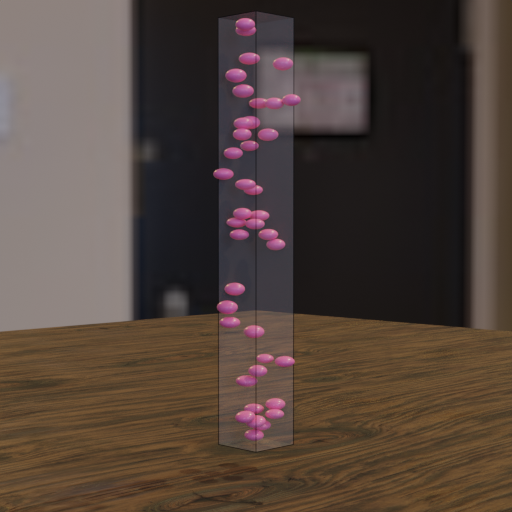
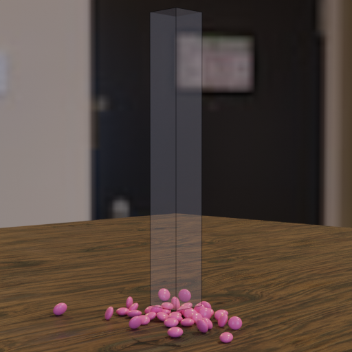
In the beginning, the particles are randomly distributed in the MeasurementVolume. In the end of the physics simulation – more specific: after our second RelaxCollisions function – all particles are located on the ground due to the simulated gravity. The MeasurementVolume doesn’t participate in the physics simulation, i.e. the boundary doesn’t affect the particles’ movement, especially doesn’t block the particles from moving out of the volume.
As can be seen, the measurement volume is represented by an elongated shape along the z axis. This is why we decide to use the feature location_z. For the moment, let’s categorize our particles in three groups, i.e. sets. We call those sets Category1, Category2 and Category3. They must fulfil the criteria IsCat1, IsCat2 and IsCat3, respectively.
process_conditions:
  feature_criteria:
    IsCat1:
      _target_: $plugins.official.InCompartment
      feature_name: location_z
      compartment_no: 1
      compartments_total: 3
      interval_length: 27
      default_return_value: False
    IsCat2:
      _target_: $plugins.official.InCompartment
      feature_name: location_z
      compartment_no: 2
      compartments_total: 3
      interval_length: 27
      default_return_value: False
    IsCat3:
      _target_: $plugins.official.InCompartment
      feature_name: location_z
      compartment_no: 3
      compartments_total: 3
      interval_length: 27
      default_return_value: False
  sets:
    Category1:
      criterion: $IsParticle and $IsCat1
    Category2:
      criterion: $IsParticle and $IsCat2
    Category3:
      criterion: $IsParticle and $IsCat3
Admittedly, we use a rather unusual categorization by creating a dependence on the feature location_z here. But, since it’s suitable for the purpose of illustration, it’s expedient in the current tutorial case. Let’s visualize, what we actually did.
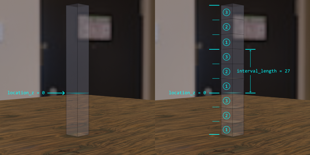
The function InCompartment, which we used to define our three criteria, can be read as follows: “Divide every <interval_length> units into <compartments_total> equidistant compartments. Check if <feature_name> lies inside compartment <compartment_no>.” For the example of IsCat1, for every object the criterion would “Divide every 27 units into 3 equidistant compartments. Check if location_z lies inside compartment 1” and – if so – return True. If the criterion is fulfilled ($IsCat1) and the checked object is a particle ($IsParticle), it will be accounted for the set Category1.
To see it in action, let’s assign different colors to the different sets. First, we add three more feature_variabilities to our list and name those PinkColor, YellowColor and GreenColor.
process_conditions:
  feature_criteria: …
  sets: …
  feature_variabilities:
    CameraNearTable: …
    InitialParticleLocation: …
    ParticleDimension: …
    ParticleWidth: …
    ParticleHeight: …
    PinkColor:
      feature_name: color
      variability:
        _target_: $plugins.official.ConstantHsvColorAsRgb
        hue: 0.95
        saturation: 0.85
    YellowColor:
      feature_name: color
      variability:
        _target_: $plugins.official.ConstantHsvColorAsRgb
        hue: 0.09
        saturation: 0.95
    GreenColor:
      feature_name: color
      variability:
        _target_: $plugins.official.ConstantHsvColorAsRgb
        hue: 0.32
        saturation: 0.77
    RenderingResolutionPercentage: …
    CyclesSamples: …
Then we trigger the update of the feature color three times by adding the corresponding TriggerFeatureUpdate to the feature_generation_steps of our synth_chain. The first trigger will only affect Category1 and change the feature color according to the definition in PinkColor. The second trigger affects Category2 and will restrict the feature color to YellowColor. The third trigger updates the feature color only for the particles in Category3 and will apply GreenColor.
synth_chain:
  feature_generation_steps:
    - _target_: $builtins.InvokeBlueprints …
    - _target_: $builtins.InvokeBlueprints …
    - _target_: $builtins.TriggerFeatureUpdate …
    - _target_: $builtins.TriggerFeatureUpdate …
    - _target_: $builtins.TriggerFeatureUpdate …
    - _target_: $builtins.TriggerFeatureUpdate …
    - _target_: $builtins.TriggerFeatureUpdate
      feature_variability_name: ParticleHeight
      affected_set_name: AllParticles
    - _target_: $builtins.TriggerFeatureUpdate
      feature_variability_name: PinkColor
      affected_set_name: Category1
    - _target_: $builtins.TriggerFeatureUpdate
      feature_variability_name: YellowColor
      affected_set_name: Category2
    - _target_: $builtins.TriggerFeatureUpdate
      feature_variability_name: GreenColor
      affected_set_name: Category3
    - _target_: $builtins.RelaxCollisions
      affected_set_name: AllParticles
      num_frames: 5
      time_scale: 10
      collision_shape: CONVEX_HULL
    - _target_: $builtins.RelaxCollisions …
    - _target_: $builtins.TriggerFeatureUpdate …
    - _target_: $builtins.TriggerFeatureUpdate …
We placed the new TriggerFeatureUpdates right after the one for ParticleHeight and the first RelaxCollisions function. The order is of major importance here! It is the reason why we speak of dynamic sets. What is dynamic about a set? Its content! The content of a set, i.e. the decision whether a particle (more general: an object of the scene) belongs to it or not, is evaluated at runtime – exactly at the moment, when the feature_generation_step is executed with respect to its sequential order in the chain, thus, in sequential relation to the other steps.
In our current case in this tutorial, it is important, that the feature color of the particles is updated first, and only then do we execute the RelaxCollisions functions, which change the feature location_z of our particles – especially the second one with gravity acting along the z axis and therefore moving particles along this direction. If we would first execute the RelaxCollisions functions and afterwards call for the TriggerFeatureUpdates of the color, only then would we also check the content of the sets and evaluate if the feature_criteria are fulfilled. Since, our three criteria IsCat1, IsCat2 and IsCat3 depend all on the feature location_z, which has almost exactly the same value for every particle after the RelaxCollisions functions (namely: floor level), this feature location_z is then rather unsuitable to distinguish between particles. Exactly this is the dynamic character about sets: They will change their content dynamically, dependent on the current “feature situation” in the 3D virtual scene. Very powerful. Use it!
For the rest of the tutorial, you should again remove the parameter dry_run, since it is not needed any further. It is always good practice to only use dry_run, if you really need it, e.g. for debugging reasons or if you just want to check how the particles move during the physics simulation, while fine-tuning parameters. The reason is that dry_run, if enabled, will not end the simulation in a clean state: The transformations in the 3D virtual scene are not actually applied. Whereas, per default after the RelaxCollisions function (dry_run: False), the transformations would indeed apply and the features are then correctly, “cleanly” set. Therefore unintentionally leaving dry_run enabled could lead to unforeseen consequences.
Let’s now execute our recipe and look at some colorful chocolate beans from our lateral perspective!
Nice! Okay, we’re almost done here. Let’s now crank it all up: More colors, different colors, more color variation, more particles!
We will assign eight different colors, so let’s first create the eight sets Category1, Category2… Category8, which are defined by the eight criteria IsCat1, IsCat2… IsCat8.
process_conditions:
  feature_criteria:
    IsCat1:
      _target_: $plugins.official.InCompartment
      feature_name: location_z
      compartment_no: 1
      compartments_total: 8
      default_return_value: False
    IsCat2:
      _target_: $plugins.official.InCompartment
      feature_name: location_z
      compartment_no: 2
      compartments_total: 8
      default_return_value: False
    IsCat3:
      _target_: $plugins.official.InCompartment
      feature_name: location_z
      compartment_no: 3
      compartments_total: 8
      default_return_value: False
    IsCat4:
      _target_: $plugins.official.InCompartment
      feature_name: location_z
      compartment_no: 4
      compartments_total: 8
      default_return_value: False
    IsCat5:
      _target_: $plugins.official.InCompartment
      feature_name: location_z
      compartment_no: 5
      compartments_total: 8
      default_return_value: False
    IsCat6:
      _target_: $plugins.official.InCompartment
      feature_name: location_z
      compartment_no: 6
      compartments_total: 8
      default_return_value: False
    IsCat7:
      _target_: $plugins.official.InCompartment
      feature_name: location_z
      compartment_no: 7
      compartments_total: 8
      default_return_value: False
    IsCat8:
      _target_: $plugins.official.InCompartment
      feature_name: location_z
      compartment_no: 8
      compartments_total: 8
      default_return_value: False
  sets:
    Category1:
      criterion: $IsParticle and $IsCat1
    Category2:
      criterion: $IsParticle and $IsCat2
    Category3:
      criterion: $IsParticle and $IsCat3
    Category4:
      criterion: $IsParticle and $IsCat4
    Category5:
      criterion: $IsParticle and $IsCat5
    Category6:
      criterion: $IsParticle and $IsCat6
    Category7:
      criterion: $IsParticle and $IsCat7
    Category8:
      criterion: $IsParticle and $IsCat8
  feature_variabilities: …
We define all the feature_criteria and new sets analogously to the example before, but this time we use a number of 8 for compartments_total and do not further specify the interval_length. The latter will default to 1.0 and will therefore be much smaller than the usual extent of each particle (see ParticleDimension as specified under feature_variabilities) – ultimately resulting in a “kind of” almost randomized color assignment. Worth mentioning, the exact location_z of each particle corresponds to its origin – in the case of our ellipsoid: its center of symmetry.
Now we specify more colors with more variation.
  feature_variabilities:
    CameraNearTable: …
    InitialParticleLocation: …
    ParticleDimension: …
    ParticleWidth: …
    ParticleHeight: …
    PinkColor:
      feature_name: color
      variability:
        _target_: $plugins.official.RandomHsvColorAsRgb
        h_min: 0.945
        h_max: 0.950
        s_min: 0.895
        s_max: 0.900
        v_min: 0.648
        v_max: 0.653
    RedColor:
      feature_name: color
      variability:
        _target_: $plugins.official.RandomHsvColorAsRgb
        h_min: 0.990
        h_max: 0.995
        s_min: 0.995
        s_max: 1.000
        v_min: 0.448
        v_max: 0.453
    OrangeColor:
      feature_name: color
      variability:
        _target_: $plugins.official.RandomHsvColorAsRgb
        h_min: 0.020
        h_max: 0.025
        s_min: 0.995
        s_max: 1.000
        v_min: 0.895
        v_max: 0.900
    YellowColor:
      feature_name: color
      variability:
        _target_: $plugins.official.RandomHsvColorAsRgb
        h_min: 0.087
        h_max: 0.092
        s_min: 0.945
        s_max: 0.950
        v_min: 0.862
        v_max: 0.867
    GreenColor:
      feature_name: color
      variability:
        _target_: $plugins.official.RandomHsvColorAsRgb
        h_min: 0.321
        h_max: 0.326
        s_min: 0.770
        s_max: 0.775
        v_min: 0.253
        v_max: 0.258
    BlueColor:
      feature_name: color
      variability:
        _target_: $plugins.official.RandomHsvColorAsRgb
        h_min: 0.622
        h_max: 0.627
        s_min: 0.846
        s_max: 0.851
        v_min: 0.547
        v_max: 0.552
    PurpleColor:
      feature_name: color
      variability:
        _target_: $plugins.official.RandomHsvColorAsRgb
        h_min: 0.716
        h_max: 0.721
        s_min: 0.801
        s_max: 0.806
        v_min: 0.348
        v_max: 0.353
    BrownColor:
      feature_name: color
      variability:
        _target_: $plugins.official.RandomHsvColorAsRgb
        h_min: 0.020
        h_max: 0.025
        s_min: 0.796
        s_max: 0.801
        v_min: 0.082
        v_max: 0.087
    RenderingResolutionPercentage: …
    CyclesSamples: …
As can be seen, we play quite a lot with the color wheel this time. Be aware that in the figure below, only the color with the average values of hue, saturation and value is shown for each feature variability. Every feature variability actually spans a 3D range for each color to allow for a little bit of variation in tone for each of the eight colors.
Last thing to do? Right: TriggerFeatureUpdates!
synth_chain:
  feature_generation_steps:
    - _target_: $builtins.InvokeBlueprints …
    - _target_: $builtins.InvokeBlueprints …
    - _target_: $builtins.TriggerFeatureUpdate …
    - _target_: $builtins.TriggerFeatureUpdate …
    - _target_: $builtins.TriggerFeatureUpdate …
    - _target_: $builtins.TriggerFeatureUpdate …
    - _target_: $builtins.TriggerFeatureUpdate
      feature_variability_name: ParticleHeight
      affected_set_name: AllParticles
    - _target_: $builtins.TriggerFeatureUpdate
      feature_variability_name: PinkColor
      affected_set_name: Category1
    - _target_: $builtins.TriggerFeatureUpdate
      feature_variability_name: RedColor
      affected_set_name: Category2
    - _target_: $builtins.TriggerFeatureUpdate
      feature_variability_name: OrangeColor
      affected_set_name: Category3
    - _target_: $builtins.TriggerFeatureUpdate
      feature_variability_name: YellowColor
      affected_set_name: Category4
    - _target_: $builtins.TriggerFeatureUpdate
      feature_variability_name: GreenColor
      affected_set_name: Category5
    - _target_: $builtins.TriggerFeatureUpdate
      feature_variability_name: BlueColor
      affected_set_name: Category6
    - _target_: $builtins.TriggerFeatureUpdate
      feature_variability_name: PurpleColor
      affected_set_name: Category7
    - _target_: $builtins.TriggerFeatureUpdate
      feature_variability_name: BrownColor
      affected_set_name: Category8
    - _target_: $builtins.RelaxCollisions …
    - _target_: $builtins.RelaxCollisions …
    - _target_: $builtins.TriggerFeatureUpdate …
    - _target_: $builtins.TriggerFeatureUpdate …
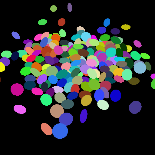
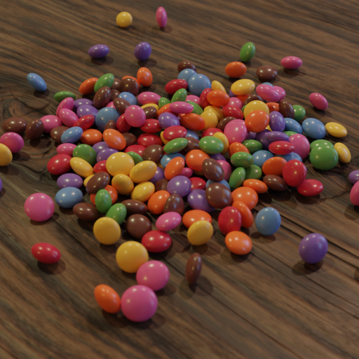
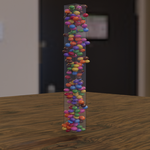
An execution of the current recipe will output the following rendered image.
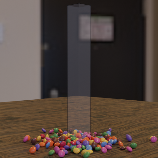
They’re looking really pretty, but when starting to nibble… 40 chocolate beans are rather a joy for a minute or two. Let’s put some more of these tasteful little things on the table! We increase the number of our Beads to 200.
blueprints:
  measurement_techniques:
  particles:
    Bead:
      geometry_prototype_name: ellipsoid
      material_prototype_name: colored_subtle
      parent: MeasurementVolume
      number: 200
Let’s finalize this tutorial: We will render out our real image and some categorical images. When creating the latter, for two of the rendering_steps, we want to focus only on the pink particles. Aww… those pink ones!
Therefore, we create one more, last feature_criteria with name IsPink and one more set with name PinkParticles.
If you ask yourself: “Why do we not easily take the already existing set Category1?” Because after all, those were the ones, to which we assigned the pink color… Our rendering_steps come in the very end: When all particles already have fallen. So, in order to filter for the pink particles, let’s not take that set, which dynamically (at the time, when we check the affected set) evaluates the feature location_z. But let’s actually define that criterion by our concrete definition of the feature, we’re looking for: pink color.
process_conditions:
  feature_criteria:
    IsCat1: …
    IsCat2: …
    IsCat3: …
    IsCat4: …
    IsCat5: …
    IsCat6: …
    IsCat7: …
    IsCat8: …
    IsPink:
      _target_: $plugins.official.InHsvRange
      feature_name: color
      h_min: 0.945
      h_max: 0.950
      s_min: 0.895
      s_max: 0.900
      v_min: 0.648
      v_max: 0.653
      default_return_value: False
  sets:
    Category1: …
    Category2: …
    Category3: …
    Category4: …
    Category5: …
    Category6: …
    Category7: …
    Category8: …
    PinkParticles:
      criterion: $IsParticle and $IsPink
  feature_variabilities: …
Now, we add three more categorical rendering steps, two of them only affecting the PinkParticles.
rendering_steps:
- _target_: $builtins.SaveState …
- _target_: $builtins.RenderParticlesTogether
rendering_mode: real
do_save_features: True
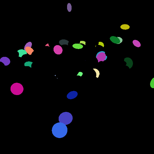
- _target_: $builtins.RenderParticlesTogether
rendering_mode: categorical
output_file_name_prefix: all_
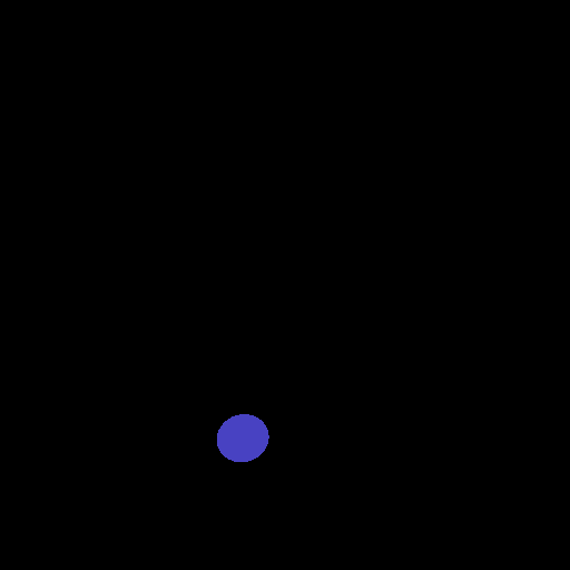
- _target_: $builtins.RenderParticlesTogether
rendering_mode: categorical
set_name_of_interest: PinkParticles
output_file_name_prefix: pink_
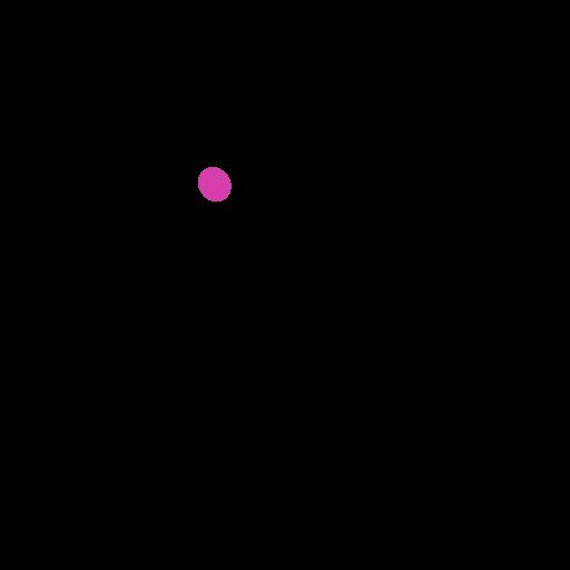
- _target_: $builtins.RenderParticlesIndividually
rendering_mode: categorical
set_name_of_interest: PinkParticles
subfolder: pink
Before we execute our recipe one last time, we increase the render samples to a number of 512.
    CyclesSamples:
      feature_name: cycles_samples
      variability:
        _target_: $builtins.Constant
        value: 512
We can find our output files of the RenderParticlesTogether steps in the locations:
output/chocBeans_table/<YYYY-MM-DD_hh-mm-ss>/run0/real/<hash>.pngoutput/chocBeans_table/<YYYY-MM-DD_hh-mm-ss>/run0/categorical/all_<hash>.pngoutput/chocBeans_table/<YYYY-MM-DD_hh-mm-ss>/run0/categorical/pink_<hash>.png
For the RenderParticlesIndividually step, the subfolder output/chocBeans_table/<YYYY-MM-DD_hh-mm-ss>/run0/categorical/pink/ contains one image for each pink particle without overlapping of other particles. Three of them are shown at the bottom row.