Synthesized Beads

In this first tutorial, we will have a look at the general concept of synthesizing particle ensembles with synthPIC2. As opposed to the minimum working example “Hello World” of the Getting Started section, you will learn to know the process of working with a SynthRecipe. The overall structure of such recipe with its main parts is roughly presented. The main goal of this brief tutorial is to get a first impression of working with synthPIC2 to produce synthesized particle data. A more in-depth description of the structure of a SynthRecipe is given in the Concepts section.

At a Glance

What We Will Learn

• The structure and creation of an executable recipe

• Understanding the content of a measurement technique prototype (=scene setup)

• Invoking blueprints, namely the measurement technique and particles

• Adapting parameters to manipulate the outcome

• Rendering our scene to visualize & quantify results

Step 1: Create and Execute Recipe

The first thing we need, is our SynthRecipe for synthPIC2, so our toolbox knows what actually needs to be done. Therefore, we create such a recipe called beads.yaml inside the recipes subfolder under our root folder of synthPIC2. Inside this file paste the following content.

beads.yaml

# Initializing and seeding
defaults:
  - BaseRecipe
  - _self_
initial_runtime_state:
  seed: 42
# Defining blueprints
blueprints:
  measurement_techniques:
    Camera:
      measurement_technique_prototype_name: default
# Procedural steps of synthetization chain
synth_chain:
  feature_generation_steps:
    - _target_: $builtins.InvokeBlueprints
      affected_set_name: AllMeasurementTechniqueBlueprints
  rendering_steps:
    - _target_: $builtins.RenderParticlesTogether
      rendering_mode: real

What we did with this short snippet is giving synthPIC2 the minimum viable recipe to setup a scene and render it. We can call it by executing the following command inside our Docker container.

python run.py --config-dir=recipes --config-name=beads

Step 2: Inspect and Understand Scene

The resulting rendered scene can be found in the image file output/beads/<YYYY-MM-DD_hh-mm-ss>/run0/real/<hash>.png under our root directory of synthPIC2.

Fascinating, isn’t it? We got an empty image!

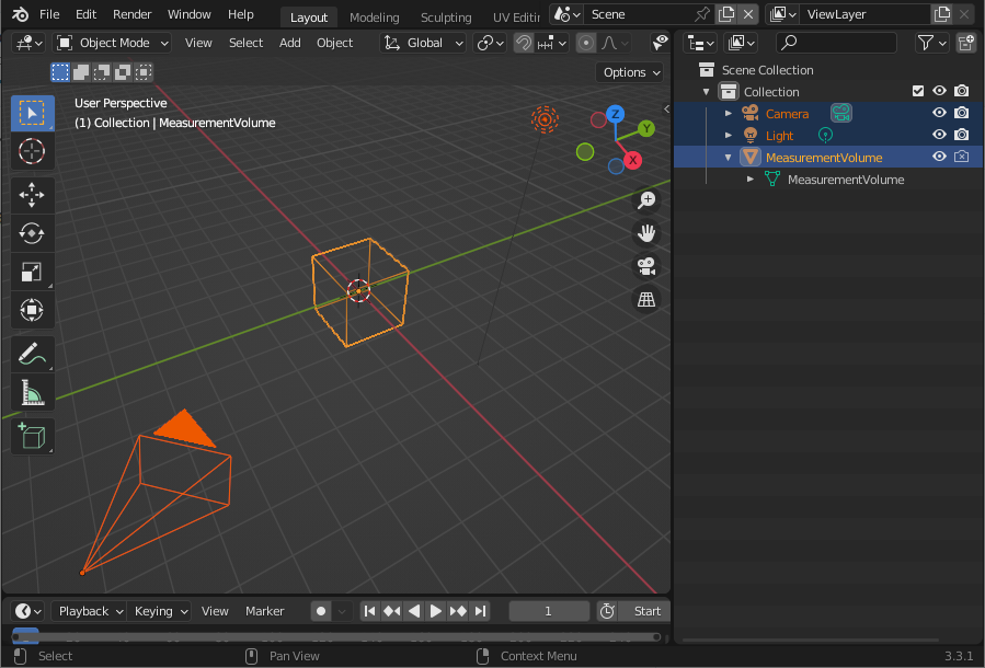
What did we actually do? Let’s have a closer look at our recipe beads.yaml. After the first 6 lines of referencing the BaseRecipe and giving a freely selectable seed for reproducibility, we build the two major blocks of the recipe: blueprints and synth_chain. Inside the blueprints, we define one measurement technique, which we call Camera. The following attribute measurement_technique_prototype_name refers to the default.blend file, which can be found inside prototype_library/measurement_techniques and which contains our scene setup for the measurement technique. When we open this file in Blender, we understand how the scene is built.

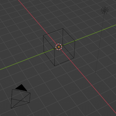
There is one light source called Light, one camera object called Camera and one cube in the coordinate origin called MeasurementVolume, which is invisible in rendering (see crossed out camera symbol, right hand side). Going back to our recipe, we see that our synth_chain defines to first execute a step for feature generation and afterwards a rendering step: First, we invoke the previously defined measurement technique blueprint by simply invoking all defined measurement techniques (we only have one) with the reference to the set AllMeasurementTechniqueBlueprints. Finally, we just capture the scene as seen by the Camera object in Blender: a photo of the coordinate origin, where the invisible MeasurementVolume cube sits.

Step 3: Bring in Particles

To make the scene more exciting, let’s bring in some particles! We do so, by adding another blueprint called Sphere. We refer to the default geometry prototype (which is a sphere) and want to have a count of 3 particles in total.

blueprints:
  measurement_techniques: …
  particles:
    Sphere:
      geometry_prototype_name: default
      number: 3

Furthermore, we state a process condition to define the allowed locations for particle placement. process_conditions can be seen as the physical boundary conditions of the system and are defined one the top-most level in the recipe, in between blueprints and synth_chain. In our case, we want the particles to be placed inside the MeasurementVolume and therefore we restrict the particles’ feature location to the boundaries of the MeasurementVolume. Since we want every location to have the same probability, we choose a uniform distribution to draw a random number from.

# Physical boundary conditions
process_conditions:
  feature_variabilities:
    ParticleLocation:
      feature_name: location
      variability:
        _target_: $builtins.UniformlyRandomLocationInMeasurementVolume

Finally, we want to use our newly defined elements and therefore need to add two more steps to our synth_chain under feature_generation_steps.

synth_chain:
  feature_generation_steps:
    - _target_: $builtins.InvokeBlueprints
      affected_set_name: AllParticleBlueprints
    - _target_: $builtins.TriggerFeatureUpdate
      feature_variability_name: ParticleLocation
      affected_set_name: AllParticles

The first new step invokes the three particles, which means to import the geometry as often as specified (here: three times) with original coordinates from their .blend file, the origin by default. Only afterwards, the particles are actually repositioned by easily triggering the update of the earlier defined feature: ParticleLocation. Note that we do not have to specify exactly, how the feature should behave. We just “trigger” the update. The reason for this is that we already defined the physical boundary condition inside process_conditions. Our extended beads.yaml recipe should now look as follows.

beads.yaml

# Initializing and seeding
defaults:
  - BaseRecipe
  - _self_
initial_runtime_state:
  seed: 42
# Defining blueprints
blueprints:
  measurement_techniques:
    Camera:
      measurement_technique_prototype_name: default
  particles:
    Sphere:
      geometry_prototype_name: default
      number: 3
# Physical boundary conditions
process_conditions:
  feature_variabilities:
    ParticleLocation:
      feature_name: location
      variability:
        _target_: $builtins.UniformlyRandomLocationInMeasurementVolume
# Procedural steps of synthetization chain
synth_chain:
  feature_generation_steps:
    - _target_: $builtins.InvokeBlueprints
      affected_set_name: AllMeasurementTechniqueBlueprints
    - _target_: $builtins.InvokeBlueprints
      affected_set_name: AllParticleBlueprints
    - _target_: $builtins.TriggerFeatureUpdate
      feature_variability_name: ParticleLocation
      affected_set_name: AllParticles
  rendering_steps:
    - _target_: $builtins.RenderParticlesTogether
      rendering_mode: real

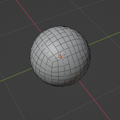
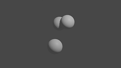
Executing the updated SynthRecipe produces the rendered image of our three particles.

Step 4: Pumping up the Scene

Okay, that was a good start! As a next step, we add some more particles by simply increasing the number when defining the particle blueprint Sphere.

blueprints:
  measurement_techniques: …
  particles:
    Sphere:
      geometry_prototype_name: default
      number: 40

We add a new feature variability to scale the particles. They should only measure 60% of the diameter of their initial standard unit size as taken from the geometry prototype default.blend file. Another feature generation step will execute the procedural step of the synth_chain to apply the resizing, i.e. triggering the update of the feature dimensions within its allowed feature variability ParticleDimension.

process_conditions:
  feature_variabilities:
    ParticleDimension:
      feature_name: dimensions
      variability:
        _target_: $builtins.UniformDistribution3dHomogeneous
        location: 0.6
        scale: 0
synth_chain:
  feature_generation_steps:
    - _target_: $builtins.TriggerFeatureUpdate
      feature_variability_name: ParticleDimension
      affected_set_name: AllParticles

We add one more feature generation step RelaxCollisions to avoid particle intersection after the random positioning inside the MeasurementVolume. Additionally, we add the attribute do_save_features to the rendering step to obtain quantitative data of our synthesized beads. The final SynthRecipe looks as follows.

beads.yaml

# Initializing and seeding
defaults:
  - BaseRecipe
  - _self_
initial_runtime_state:
  seed: 42
# Defining blueprints
blueprints:
  measurement_techniques:
    Camera:
      measurement_technique_prototype_name: default
  particles:
    Sphere:
      geometry_prototype_name: default
      number: 40
# Physical boundary conditions
process_conditions:
  feature_variabilities:
    ParticleLocation:
      feature_name: location
      variability:
        _target_: $builtins.UniformlyRandomLocationInMeasurementVolume
    ParticleDimension:
      feature_name: dimensions
      variability:
        _target_: $builtins.UniformDistribution3dHomogeneous
        location: 0.6
        scale: 0
# Procedural steps of synthetization chain
synth_chain:
  feature_generation_steps:
    - _target_: $builtins.InvokeBlueprints
      affected_set_name: AllMeasurementTechniqueBlueprints
    - _target_: $builtins.InvokeBlueprints
      affected_set_name: AllParticleBlueprints
    - _target_: $builtins.TriggerFeatureUpdate
      feature_variability_name: ParticleLocation
      affected_set_name: AllParticles
    - _target_: $builtins.TriggerFeatureUpdate
      feature_variability_name: ParticleDimension
      affected_set_name: AllParticles
    - _target_: $builtins.RelaxCollisions
      affected_set_name: AllParticles
      collision_shape: SPHERE
  rendering_steps:
    - _target_: $builtins.RenderParticlesTogether
      rendering_mode: real
      do_save_features: True

We execute the recipe one more time.

python run.py --config-dir=recipes --config-name=beads

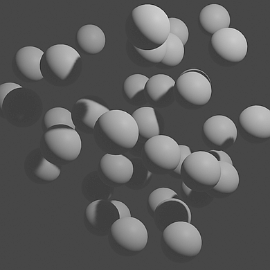
Now, we can open our resulting file output/beads/<YYYY-MM-DD_hh-mm-ss>/run0/real/<hash>.png and look at a nice illustration of our first rendered particle ensemble.

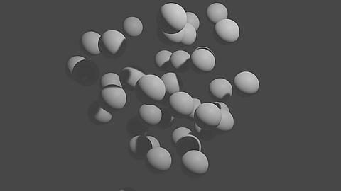
The accompanying file particle_features.csv in the same folder gives insights about the particles’ individual ID (hash), the name of the blueprint from which they were invoked, their dimension and exact position as well as further features of each particle.