SEM: More Rendering Modes & Production Scale Use
This tutorial demonstrates a real use-case: the generation of data for the training of a neural network for particle detection in secondary electron microscopy (SEM) images. To train the network, we need a lot of lifelike and heterogeneous data, so that the network is applicable to real images and learns to generalize.
Therefore, we create a recipe with a lot of feature variabilities, so that we can introduce some randomness in the generated images. While we’re at it, we demonstrate a few more rendering modes, to have some more versatile forms of ground truth available for our training.
Since this is an advanced tutorial, we assume that you are already familiar with the basic concepts of the toolbox.
At a Glance

What You Will Learn
Recap of basic rendering modes:
realandcategoricalMore exotic rendering modes:
stylized,stylized_xray,normal_mapanddepth_mapHow to create a recipe that is versatile enough to create a large and heterogeneous data set, suitable for the training of a particle detection network.
Recipe
The recipe for this tutorial can be found in recipes/spheres_sem.yaml:
defaults:
  - BaseRecipe
  - _self_

initial_runtime_state:
  time: 0.0
  seed: 42
blueprints:
  measurement_techniques:
    SEM:
      measurement_technique_prototype_name: secondary_electron_microscope
      background_material_prototype_name: sem_patchy_silicone
  particles:
    Bead:
      geometry_prototype_name: sphere
      material_prototype_name: sem_polystyrene
      parent: MeasurementVolume
      number: 600
process_conditions:
  feature_variabilities:
    ParticleDimension:
      feature_name: dimensions
      variability:
        _target_: $builtins.UniformDistribution3dHomogeneous
        location: 5
        scale: 2
    ParticleSubdivisions:
      feature_name: subdivisions
      variability:
        _target_: $builtins.Constant
        value: 1
    InitialParticleLocation:
      feature_name: location
      variability:
        _target_: $builtins.UniformlyRandomLocationInMeasurementVolume
    NoiseThreshold:
      feature_name: noise_threshold
      variability:
        _target_: $builtins.UniformDistributionNdHomogeneous
        location: 0.05
        scale: 0.05
        num_dimensions: 1
    Defocus:
      feature_name: defocus
      variability:
        _target_: $builtins.UniformDistributionNdHomogeneous
        location: 0.2
        scale: 0.3
        num_dimensions: 1
    IlluminationStrength:
      feature_name: illumination_strength
      variability:
        _target_: $builtins.UniformDistributionNdHomogeneous
        location: 1
        scale: 2
        num_dimensions: 1
    BackgroundPatchScale:
      feature_name: patch_scale
      variability:
        _target_: $builtins.UniformDistributionNdHomogeneous
        location: 25
        scale: 75
        num_dimensions: 1
    BackgroundPatchSeed:
      feature_name: patch_seed
      variability:
        _target_: $builtins.Constant
        value: ${initial_runtime_state.seed}
synth_chain:
  feature_generation_steps:
    - _target_: $builtins.InvokeBlueprints
      affected_set_name: AllMeasurementTechniqueBlueprints
    - _target_: $builtins.InvokeBlueprints
      affected_set_name: AllParticleBlueprints
    - _target_: $builtins.TriggerFeatureUpdate
      feature_variability_name: ParticleDimension
      affected_set_name: AllParticles
    - _target_: $builtins.TriggerFeatureUpdate
      feature_variability_name: ParticleSubdivisions
      affected_set_name: AllParticles
    - _target_: $builtins.TriggerFeatureUpdate
      feature_variability_name: InitialParticleLocation
      affected_set_name: AllParticles
    - _target_: $builtins.RelaxCollisions
      affected_set_name: AllParticles
      collision_shape: SPHERE
      use_gravity: True
      gravity:
        - 0
        - 0
        - -100
      num_frames: 250
    - _target_: $builtins.TriggerFeatureUpdate
      feature_variability_name: Defocus
      affected_set_name: AllMeasurementTechniques
    - _target_: $builtins.TriggerFeatureUpdate
      feature_variability_name: NoiseThreshold
      affected_set_name: AllMeasurementTechniques
    - _target_: $builtins.TriggerFeatureUpdate
      feature_variability_name: IlluminationStrength
      affected_set_name: AllMeasurementTechniques
    - _target_: $builtins.TriggerFeatureUpdate
      feature_variability_name: BackgroundPatchScale
      affected_set_name: AllMeasurementTechniques
    - _target_: $builtins.TriggerFeatureUpdate
      feature_variability_name: BackgroundPatchSeed
      affected_set_name: AllMeasurementTechniques
  rendering_steps:
    - _target_: $builtins.SaveState
      name: state
    - _target_: $builtins.RenderParticlesTogether
      rendering_mode: real
    - _target_: $builtins.RenderParticlesTogether
      rendering_mode: categorical
    - _target_: $builtins.RenderParticlesTogether
      rendering_mode: depth_map
    - _target_: $builtins.RenderParticlesTogether
      rendering_mode: normal_map
    - _target_: $builtins.RenderParticlesTogether
      rendering_mode: stylized
    - _target_: $builtins.RenderParticlesTogether
      rendering_mode: stylized_xray
Step 1: Simulating Scanning Electron Microscopy (SEM)
To achieve the style of SEM images, we not only have to specify a suitable measurement technique prototype, but we need suitable material prototypes as well:
...
blueprints:
  measurement_techniques:
    SEM:
      measurement_technique_prototype_name: secondary_electron_microscope
      background_material_prototype_name: sem_patchy_silicone
  particles:
    Bead:
      geometry_prototype_name: sphere
      material_prototype_name: sem_polystyrene
      parent: MeasurementVolume
      number: 600
Note
Blender was not made to simulate electrons. This means that we have to fake the SEM style using subsurface scattering.
Step 2: Feature Variabilities
As mentioned before, this recipe makes extensive use of feature variabilities. For the sake of brevity, we will go over them just briefly.
...
  ParticleDimension:
    feature_name: dimensions
    variability:
      _target_: $builtins.UniformDistribution3dHomogeneous
      location: 5
      scale: 2
...
Although unrealistic for real particle systems, we scale our particles according to a uniform distribution, as not to create a bias towards a certain particle size.
...
  ParticleSubdivisions:
      feature_name: subdivisions
      variability:
        _target_: $builtins.Constant
        value: 1
...
The used geometry prototype has quite a high resolution. Since we’re only dealing with spheres (and actually lots of them), we can reduce the number of subdivisions, to speed up the upcoming physics simulation and the rendering.
...
  InitialParticleLocation:
    feature_name: location
    variability:
      _target_: $builtins.UniformlyRandomLocationInMeasurementVolume
...
Although later on, we will use a small physics simulation, to place our particles, we initialize their position, by distributing them evenly in the measurement volume.
...
  NoiseThreshold:
    feature_name: noise_threshold
    variability:
      _target_: $builtins.UniformDistributionNdHomogeneous
      location: 0.05
      scale: 0.05
      num_dimensions: 1
...
This feature variability randomizes the noise threshold of Blender’s Cycles rendering engine through our measurement technique. Here, it is used to control the noise of the resulting images, to match the noisiness of real SEM images.
...
  Defocus:
    feature_name: defocus
    variability:
      _target_: $builtins.UniformDistributionNdHomogeneous
      location: 0.2
      scale: 0.3
      num_dimensions: 1
...
To vary the amount of blur, which can occur in SEM images, we add variation to the defocus feature of our measurement technique, which controls the depth of field of a camera in Blender.
...
  IlluminationStrength:
    feature_name: illumination_strength
    variability:
      _target_: $builtins.UniformDistributionNdHomogeneous
      location: 1
      scale: 2
      num_dimensions: 1
...
Since the brightness of SEM images is very dependent on the operator, we introduce some variation. The varied feature controls a light source in our measurement technique.
...
  BackgroundPatchScale:
    feature_name: patch_scale
    variability:
      _target_: $builtins.UniformDistributionNdHomogeneous
      location: 25
      scale: 75
      num_dimensions: 1
...
The utilized measurement technique allows us to enable a background plane, which acts as substrate for our particles. The sem_patchy_silicone material prototype that we assigned is a procedural material and features a lot of small patches. Here, we introduce some variation to the scale of these patches.
...
  BackgroundPatchSeed:
    feature_name: patch_seed
    variability:
      _target_: $builtins.Constant
      value: ${initial_runtime_state.seed}
...
To avoid that our substrate is too similar for images with similar patch_scale values, we tie the random seed of the substrate material to our global random seed.
Step 3: Feature Generation Steps
Most feature generation steps of the recipe should already be familiar from other tutorials, so we will not elaborate upon them here, with exception of the RelaxCollisions step, since we will reference it in Step 5 of this tutorial.
...
synth_chain:
  feature_generation_steps:
    ...
    - _target_: $builtins.RelaxCollisions
      affected_set_name: AllParticles
      collision_shape: SPHERE
      use_gravity: True
      gravity:
        - 0
        - 0
        - -100
      num_frames: 250
    ...
...
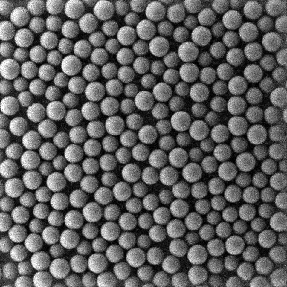
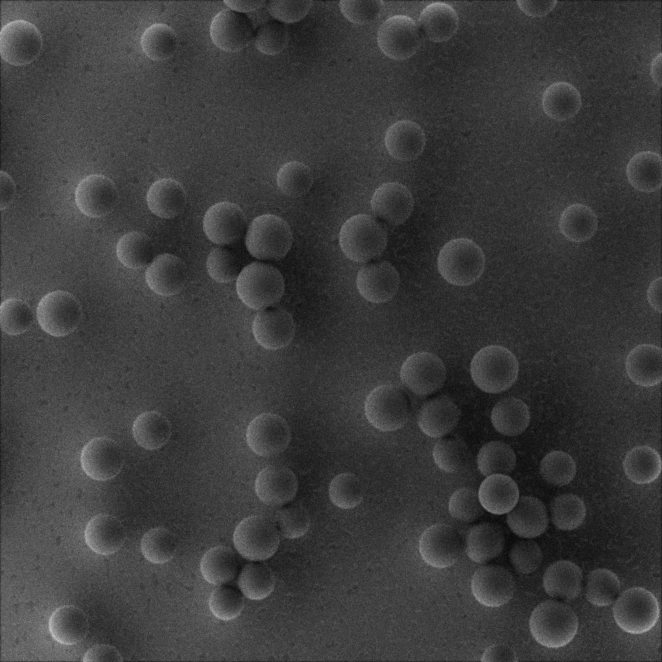
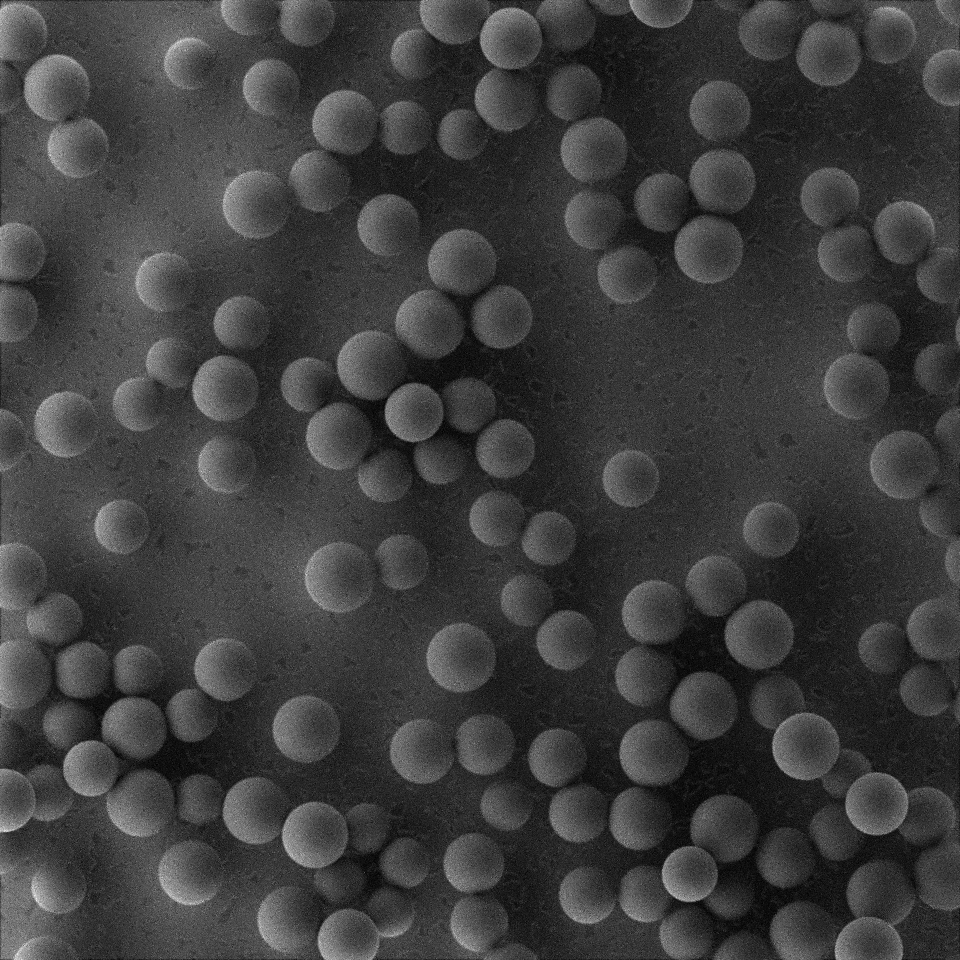
The noteworthy parameter here is the third element of the gravity parameter (-100). We will use it to create a more loose or more dense packing of our particle heap. Since the gravity of this feature generation step is not accessible as a feature, we cannot apply a feature variability. However, we can override the value for different executions of the recipe as part of a multirun (see step 5).
Step 4: Rendering Steps
...
    - _target_: $builtins.SaveState
      name: state
...
Saves the scene as a Blender file. The ultimate ground truth.
...
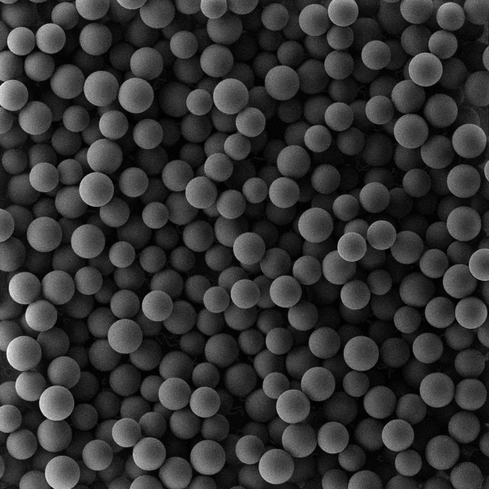
- _target_: $builtins.RenderParticlesTogether
rendering_mode: real
...
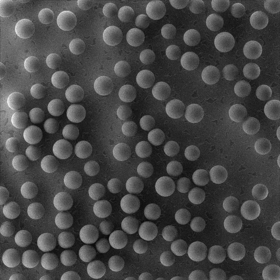
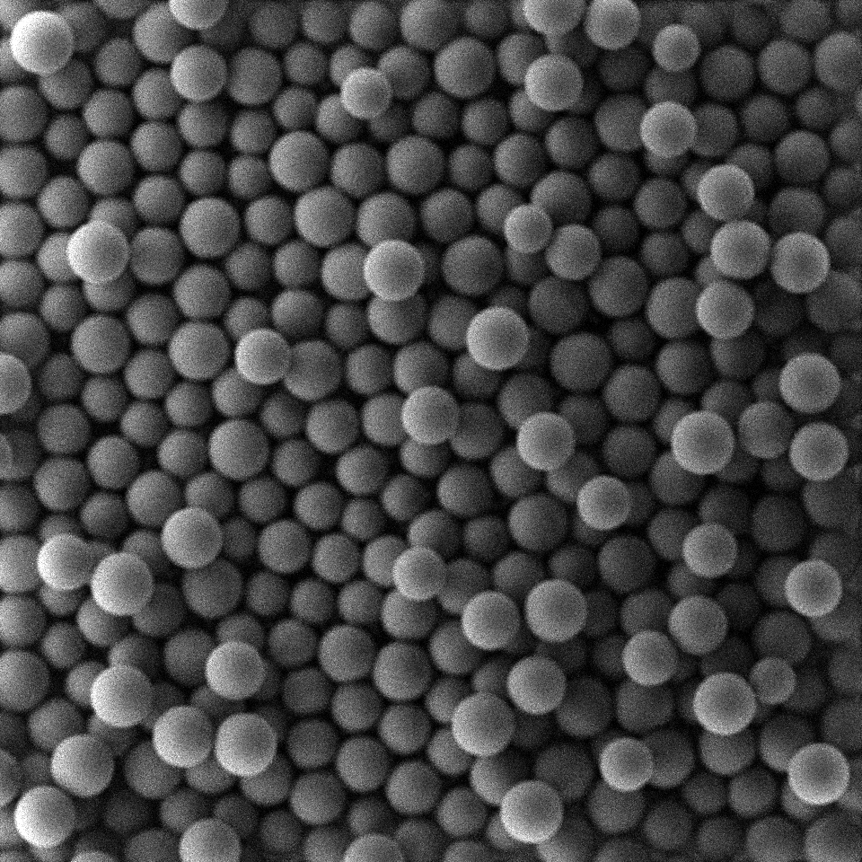
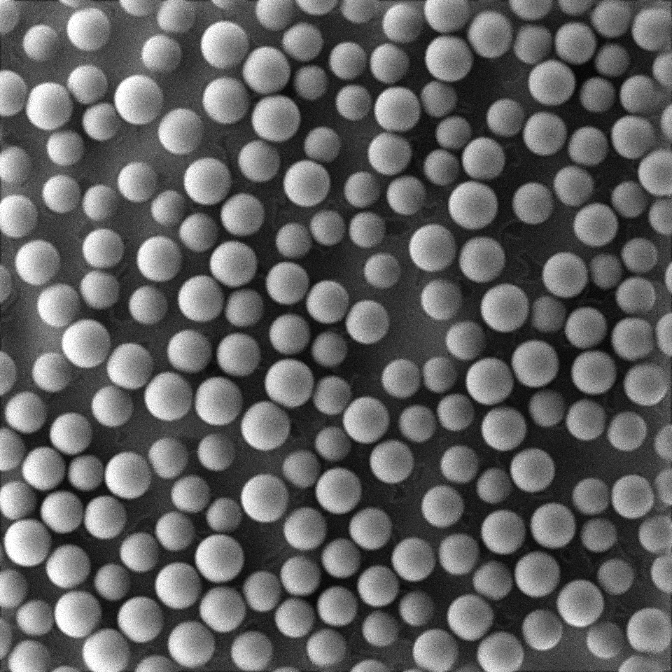
Renders a lifelike SEM image.
...
    - _target_: $builtins.RenderParticlesTogether
      rendering_mode: categorical
...
Renders a categorical image, where pixels of a certain color represent a particle.
...
    - _target_: $builtins.RenderParticlesTogether
      rendering_mode: depth_map
...
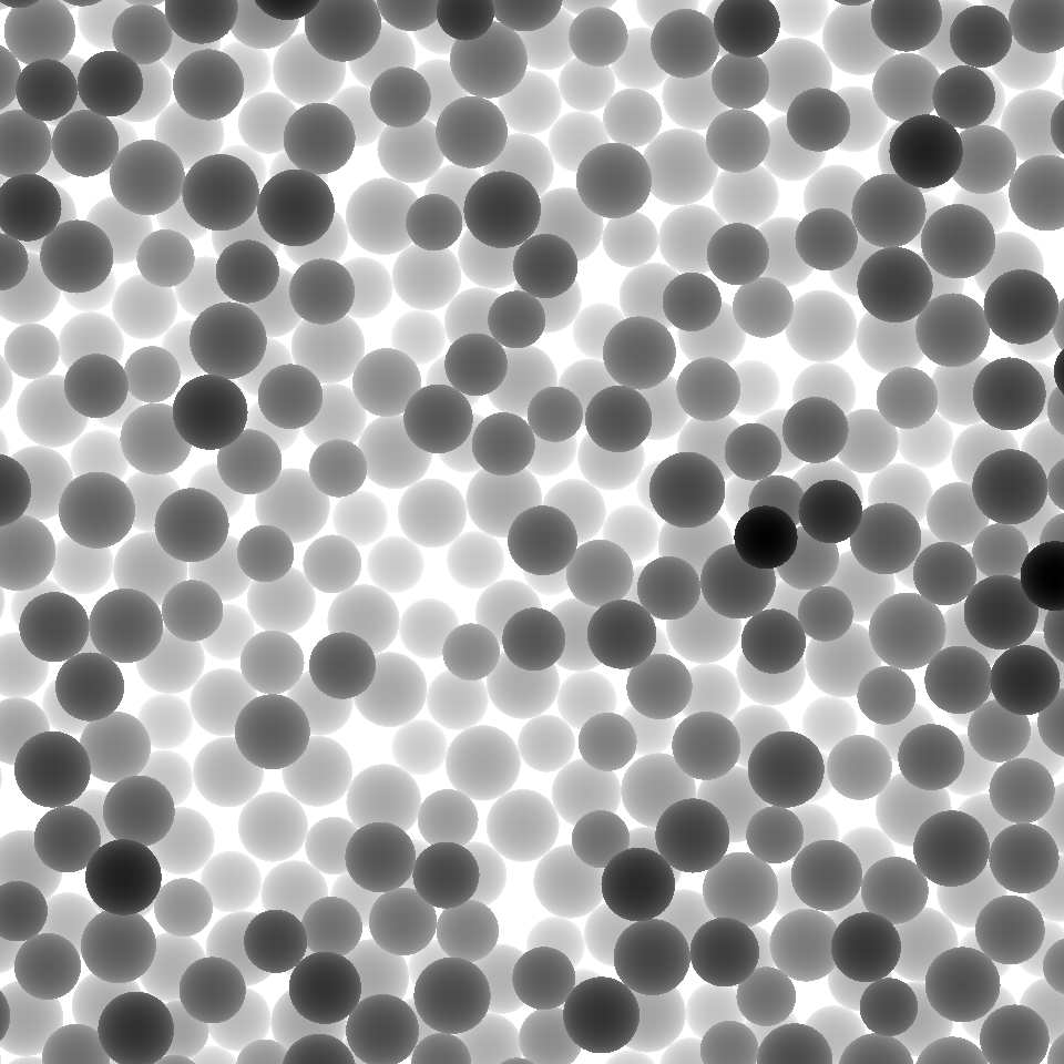
Renders a depth map, where each pixel is color-coded based on the relative distance of the underlying geometry to the camera. Darker pixels are closer to the camera than lighter pixels. Despite being 2D, this representation holds some 3D information.
...
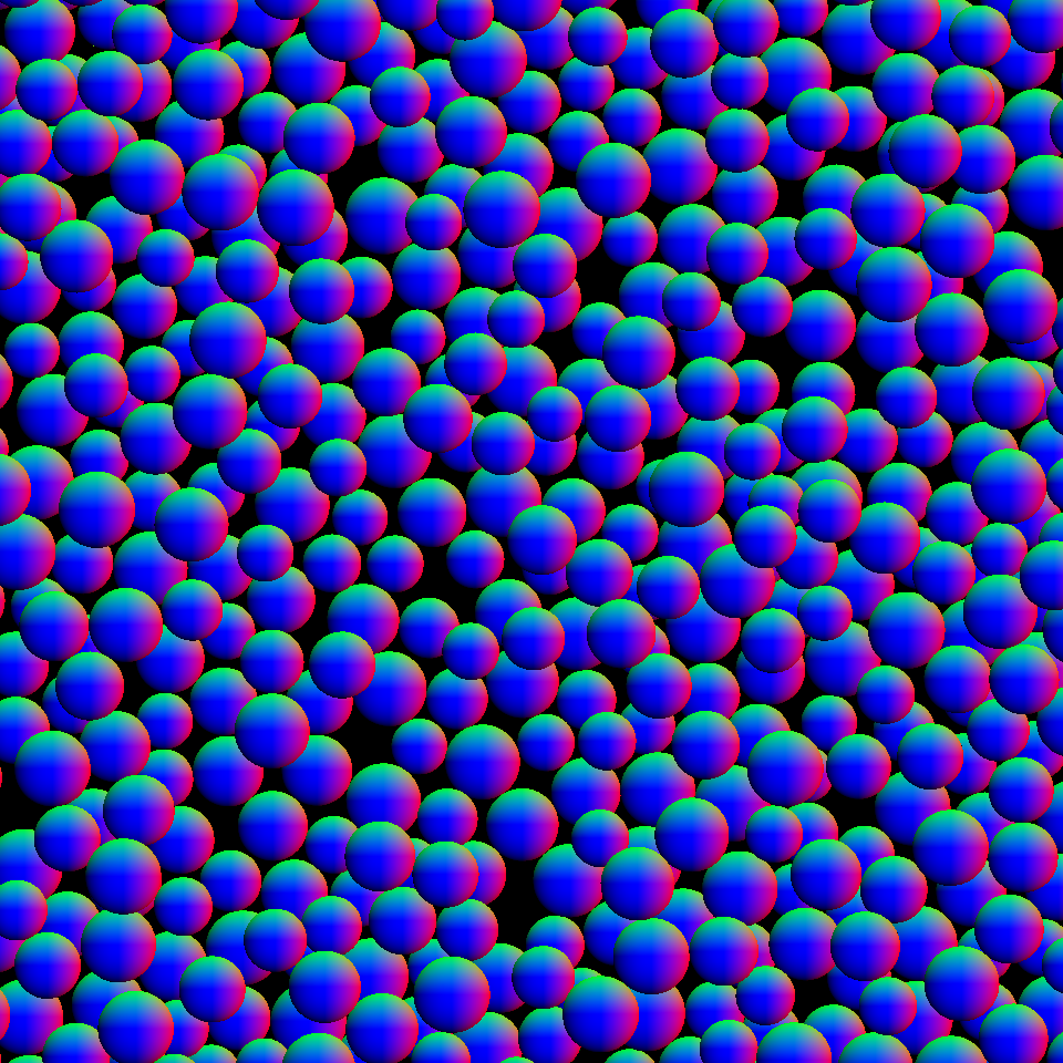
- _target_: $builtins.RenderParticlesTogether
rendering_mode: normal_map
...
Renders a normal map, where each pixel is color-coded based on the normal vector of the underlying geometry. Each color channel represents a spatial dimension. Despite being 2D, this representation holds some 3D information.
...
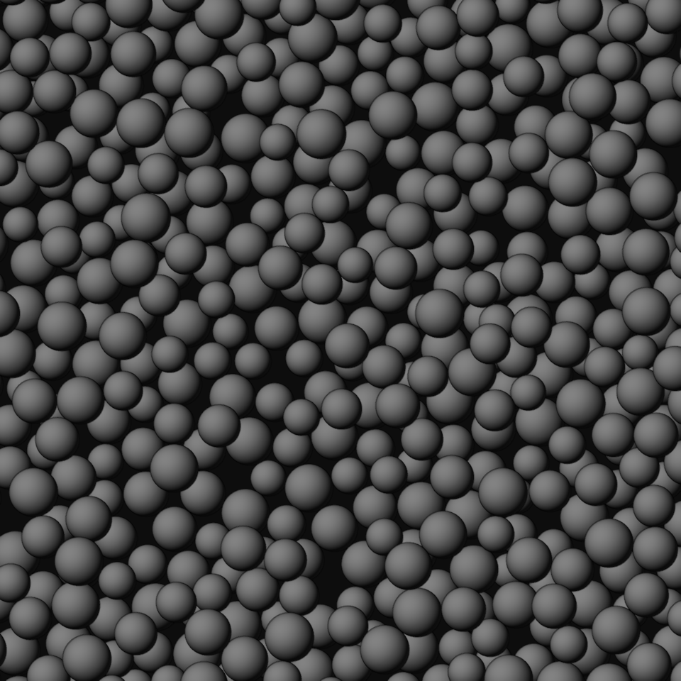
- _target_: $builtins.RenderParticlesTogether
rendering_mode: stylized
...
This render mode uses a generic material and lighting. Therefore, it is very universal but abstract.
...
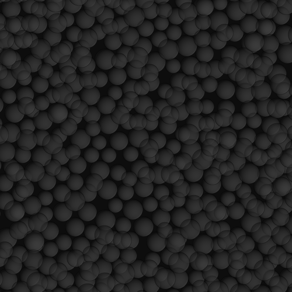
- _target_: $builtins.RenderParticlesTogether
rendering_mode: stylized_xray
...
The same as the stylized rendering mode, but with transparency.
Step 5: Multirun: Producing a Lot of Data
Now that we completed our recipe, we can use it to create a lifelike image and the associated ground truth representations. However, to train a neural network, we need a whole stack of training samples. Since we don’t want to write many recipes, we will leverage the power of the --multirun command-line parameter. Since want to be able to look up the overrides that we are using in a few months from now, we create a small bash script (see recipes/secondary_electron_microscopy_multirun.sh):
#!/usr/bin/env bash

temp=$( realpath "$0"  )
script_directory=$( dirname "$temp" )

cd $script_directory/..

python run.py \
    --config-dir=recipes \
    --config-name=secondary_electron_microscopy \
    --multirun \
    blueprints.particles.Bead.number=100,200,300,400,500,600 \
    initial_runtime_state.seed=range\(15\) \
    synth_chain.feature_generation_steps.5.gravity.2=-100,-10000
The script consists of two parts. First, it changes into the base directory of the toolbox (independently from the directory it was called from). Secondly, it executes a multirun with three overrides:
blueprints.particles.Bead.number=100,200,300,400,500,600: Here we vary the number of particles, by iterating a list of six values, so that we yield images with more or less coverage.initial_runtime_state.seed=range\(15\): Here we vary the random seed in the range from 0 to 14, to get different values for the feature variabilities that we defined in Step 2 of this tutorial. Note the use of\to escape the parentheses.synth_chain.feature_generation_steps.5.gravity.2=-100,-10000: Here we vary the third element (z coordinate) of thegravityparameter of the sixth feature generation step (RelaxCollisions, see Step 3 of this tutorial).
Since a multirun executes all permutations of the overrides, we can calculate the number of resulting runs:
(6 possible numbers of particles) x (15 possible random seeds) x (2 possible gravities) = 180 runs
To get a feeling for the heterogeneity of the resulting data, let us examine a few examples:
Note
We execute the shell script inside our Docker container that is running Linux, so it will work on any host operating system.